5 Tidyverse R
Hadley Wickham and Garrett Grolemund, in their excellent and freely available book R for Data Science, promote the concept of “tidy data.” The Tidyverse collection of R packages attempt to realize this concept in concrete libraries.
In brief, tidy data carefully separates variables (the columns of a table, also called features or fields) from observations (the rows of a table, also called samples). At the intersection of these two, we find values, one data item (datum) in each cell. Unfortunately, the data we encounter is often not arranged in this useful way, and it requires normalization. In particular, what are really values are often represented either as columns or as rows instead. To demonstrate what this means, let us consider an example (a small elementary school class).
library(tidyverse)
# inline reading, tibble version
students <- tribble(
  ~'Last Name', ~'First Name', ~'4th Grade', ~'5th Grade', ~'6th Grade',
  "Johnson", "Mia", "A", "B+", "A-",
  "Lopez", "Liam", "B", "B", "A+",
  "Lee", "Isabella", "C", "C-", "B-",
  "Fisher", "Mason", "B", "B-", "C+",
  "Gupta", "Olivia", "B", "A+", "A",
  "Robinson", "Sophia", "A+", "B-", "A"
)
students
#> # A tibble: 6 x 5
#>   `Last Name` `First Name` `4th Grade` `5th Grade`
#>   <chr>       <chr>        <chr>       <chr>
#> 1 Johnson     Mia          A           B+
#> 2 Lopez       Liam         B           B
#> 3 Lee         Isabella     C           C-
#> 4 Fisher      Mason        B           B-
#> 5 Gupta       Olivia       B           A+
#> 6 Robinson    Sophia       A+          B-
#> # ... with 1 more variable: 6th Grade <chr>
This view of the data is easy for humans to read. We can see trends in the scores each student received over several years of education. Moreover, this format might lend itself to useful visualizations fairly easily:
# Generic conversion of letter grades to numbers
recodes.str <- "'A+'=4.3;'A'=4;'A-'=3.7;'B+'=3.3;'B'=3;'B-'=2.7;'C+'=2.3;'C'= 2;'C-'=1.7"
students$`4th Grade` <- car::recode(students$`4th Grade`, recodes.str)
students$`5th Grade` <- car::recode(students$`5th Grade`, recodes.str)
students$`6th Grade` <- car::recode(students$`6th Grade`, recodes.str)

# create plot
matplot(t(students[,c(3:5)]), type = "b", pch = 11:16, col = 2:7, xaxt="n", ylab="")
Axis(labels = names(students)[3:5], side=1, at = 1:3)
legend(1.2, 3, paste(substr(x = students$`Last Name`, 1, 1), students$`First Name`, sep = ". "),
       pch = 11:16, col = 2:7)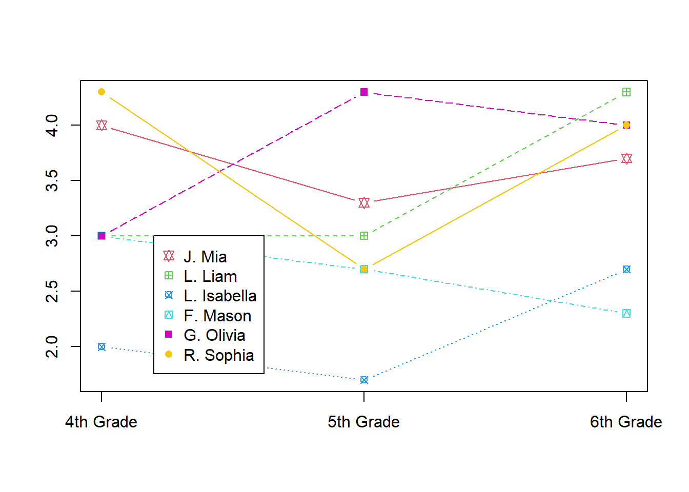
This data layout exposes its limitations once the class advances to 7th grade, or if we were to obtain 3rd grade information. To accommodate such additional data, we would need to change the number and position of columns, not simply add additional rows. It is natural to make new observations or identify new samples (rows) but usually awkward to change the underlying variables (columns).
The particular class level (e.g. 4th grade) that a letter grade pertains to is, at heart, a value, not a variable. Another way to think of this is in terms of independent variables versus dependent variables, or in machine learning terms, features versus target. In some ways, the class level might correlate with or influence the resulting letter grade; perhaps the teachers at the different levels have different biases, or children of a certain age lose or gain interest in schoolwork, for example.
For most analytic purposes, this data would be more useful if we made it tidy (normalized) before further processing. In Base R, the reshape2::melt() method can perform this tidying. We pin some of the columns as id_vars, and we set a name for the combined columns as a variable and the letter grade as a single new column.
reshape2::melt(data = students, id=c("Last Name", "First Name"))
#>    Last Name First Name  variable value
#> 1    Johnson        Mia 4th Grade   4.0
#> 2      Lopez       Liam 4th Grade   3.0
#> 3        Lee   Isabella 4th Grade   2.0
#> 4     Fisher      Mason 4th Grade   3.0
#> 5      Gupta     Olivia 4th Grade   3.0
#> 6   Robinson     Sophia 4th Grade   4.3
#> 7    Johnson        Mia 5th Grade   3.3
#> 8      Lopez       Liam 5th Grade   3.0
#> 9        Lee   Isabella 5th Grade   1.7
#> 10    Fisher      Mason 5th Grade   2.7
#> 11     Gupta     Olivia 5th Grade   4.3
#> 12  Robinson     Sophia 5th Grade   2.7
#> 13   Johnson        Mia 6th Grade   3.7
#> 14     Lopez       Liam 6th Grade   4.3
#> 15       Lee   Isabella 6th Grade   2.7
#> 16    Fisher      Mason 6th Grade   2.3
#> 17     Gupta     Olivia 6th Grade   4.0
#> 18  Robinson     Sophia 6th Grade   4.0
Within the Tidyverse, specifically within the tidyr package, there is a function pivot_longer() that is similar to Base R’s reshape2::melt(). The aggregation names and values have parameters spelled names_to= and values_to=, but the operation is the same:
s.l <- students %>%
 pivot_longer(c('4th Grade', '5th Grade', '6th Grade'),
 names_to = "Level",
 values_to = "Score")
s.l
#> # A tibble: 18 x 4
#>    `Last Name` `First Name` Level     Score
#>    <chr>       <chr>        <chr>     <dbl>
#>  1 Johnson     Mia          4th Grade   4
#>  2 Johnson     Mia          5th Grade   3.3
#>  3 Johnson     Mia          6th Grade   3.7
#>  4 Lopez       Liam         4th Grade   3
#>  5 Lopez       Liam         5th Grade   3
#>  6 Lopez       Liam         6th Grade   4.3
#>  7 Lee         Isabella     4th Grade   2
#>  8 Lee         Isabella     5th Grade   1.7
#>  9 Lee         Isabella     6th Grade   2.7
#> 10 Fisher      Mason        4th Grade   3
#> 11 Fisher      Mason        5th Grade   2.7
#> 12 Fisher      Mason        6th Grade   2.3
#> 13 Gupta       Olivia       4th Grade   3
#> 14 Gupta       Olivia       5th Grade   4.3
#> 15 Gupta       Olivia       6th Grade   4
#> 16 Robinson    Sophia       4th Grade   4.3
#> 17 Robinson    Sophia       5th Grade   2.7
#> 18 Robinson    Sophia       6th Grade   4
The simple example above gives you a first feel for tidying tabular data. To reverse the tidying operation that moves variables (columns) to values (rows), the pivot_wider() function in tidyr can be used. In Base R there are several related methods on data frames, including reshape::cast() and reshape2::dcast().
s.l %>%
  pivot_wider(names_from = Level, values_from = Score)
#> # A tibble: 6 x 5
#>   `Last Name` `First Name` `4th Grade` `5th Grade`
#>   <chr>       <chr>              <dbl>       <dbl>
#> 1 Johnson     Mia                  4           3.3
#> 2 Lopez       Liam                 3           3
#> 3 Lee         Isabella             2           1.7
#> 4 Fisher      Mason                3           2.7
#> 5 Gupta       Olivia               3           4.3
#> 6 Robinson    Sophia               4.3         2.7
#> # ... with 1 more variable: 6th Grade <dbl>
5.1 The tibble
Tibbles inherits the attributes of a data frame and enhances some of them. The tibble is the central data structure for a set of packages known as the tidyverse.
Tibbles when printed out returns:
- the first 10 rows and
- all the columns that can fit on screen and
- column types.
5.1.1 Importing data
The functions read_csv(), read_delim(), read_excel_csv(), read_tsv() are used to import data.
# loading package
library(readr)

# reading data
gapminder <- read_delim(file = 'data/gapminder_ext_UTF-8.txt',
                        delim = "\t",
                        col_names = T,
                        locale = locale(decimal_mark = ",",  encoding = "UTF-8"))
head(gapminder, 3)
#> # A tibble: 3 x 8
#>   country     continent  year lifeExp      pop gdpPercap
#>   <chr>       <chr>     <dbl>   <dbl>    <dbl>     <dbl>
#> 1 Afghanistan Asia       1952    28.8  8425333      779.
#> 2 Afghanistan Asia       1957    30.3  9240934      821.
#> 3 Afghanistan Asia       1962    32.0 10267083      853.
#> # ... with 2 more variables: country_hun <chr>,
#> #   continent_hun <chr>

# class checking
class(gapminder)
#> [1] "spec_tbl_df" "tbl_df"      "tbl"         "data.frame"

# checking for data frame
is.data.frame(gapminder)
#> [1] TRUE
5.1.2 Tibbles are data frames
Since Tibbles are data frames, functions which operate on data frames also operate on them.
head(gapminder, 3)
#> # A tibble: 3 x 8
#>   country     continent  year lifeExp      pop gdpPercap
#>   <chr>       <chr>     <dbl>   <dbl>    <dbl>     <dbl>
#> 1 Afghanistan Asia       1952    28.8  8425333      779.
#> 2 Afghanistan Asia       1957    30.3  9240934      821.
#> 3 Afghanistan Asia       1962    32.0 10267083      853.
#> # ... with 2 more variables: country_hun <chr>,
#> #   continent_hun <chr>
tail(gapminder, 3)
#> # A tibble: 3 x 8
#>   country  continent  year lifeExp      pop gdpPercap
#>   <chr>    <chr>     <dbl>   <dbl>    <dbl>     <dbl>
#> 1 Zimbabwe Africa     1997    46.8 11404948      792.
#> 2 Zimbabwe Africa     2002    40.0 11926563      672.
#> 3 Zimbabwe Africa     2007    43.5 12311143      470.
#> # ... with 2 more variables: country_hun <chr>,
#> #   continent_hun <chr>
nrow(gapminder)
#> [1] 1704
ncol(gapminder)
#> [1] 8
summary(gapminder)
#>    country           continent              year
#>  Length:1704        Length:1704        Min.   :1952
#>  Class :character   Class :character   1st Qu.:1966
#>  Mode  :character   Mode  :character   Median :1980
#>                                        Mean   :1980
#>                                        3rd Qu.:1993
#>                                        Max.   :2007
#>     lifeExp           pop              gdpPercap
#>  Min.   :23.60   Min.   :6.001e+04   Min.   :   241.2
#>  1st Qu.:48.20   1st Qu.:2.794e+06   1st Qu.:  1202.1
#>  Median :60.71   Median :7.024e+06   Median :  3531.8
#>  Mean   :59.47   Mean   :2.960e+07   Mean   :  7215.3
#>  3rd Qu.:70.85   3rd Qu.:1.959e+07   3rd Qu.:  9325.5
#>  Max.   :82.60   Max.   :1.319e+09   Max.   :113523.1
#>  country_hun        continent_hun
#>  Length:1704        Length:1704
#>  Class :character   Class :character
#>  Mode  :character   Mode  :character
#>
#>
#>
5.1.3 Exporting data
The functions write_csv(), write_delim(), write_excel_csv(), write_tsv() are used to export data. To export Tibbles, they have first to be converted into data frames.
# exporting Tibbles
write_delim(x = data.frame(gapminder), delim = " ", file = 'output/data/gapminderfixedwidth.txt')
write_csv(x = data.frame(gapminder), file = 'output/data/gapminder_csv.txt')
write_tsv(x = data.frame(gapminder), file = 'output/data/gapminder_tsv.txt')

# checking if files exist?
file.exists(c('output/data/gapminderfixedwidth.txt', 'output/data/gapminder_csv.txt', 'output/data/gapminder_tsv.txt'))
#> [1] TRUE TRUE TRUE

# removing files
file.remove(c('output/data/gapminderfixedwidth.txt', 'output/data/gapminder_csv.txt', 'output/data/gapminder_tsv.txt'))
#> [1] TRUE TRUE TRUE
5.1.4 Check for tibble
Tibbles come from the package tibble.
The function is_tibble() is used to check for tibble.
The function glimpse() is a better option of str().
# loading tibble
library(tibble)

# glimpse() a better option to str()
glimpse(gapminder)
#> Rows: 1,704
#> Columns: 8
#> $ country       <chr> "Afghanistan", "Afghanistan", "Afgha~
#> $ continent     <chr> "Asia", "Asia", "Asia", "Asia", "Asi~
#> $ year          <dbl> 1952, 1957, 1962, 1967, 1972, 1977, ~
#> $ lifeExp       <dbl> 28.801, 30.332, 31.997, 34.020, 36.0~
#> $ pop           <dbl> 8425333, 9240934, 10267083, 11537966~
#> $ gdpPercap     <dbl> 779.4453, 820.8530, 853.1007, 836.19~
#> $ country_hun   <chr> "Afganisztán", "Afganisztán", "Afgan~
#> $ continent_hun <chr> "Ázsia", "Ázsia", "Ázsia", "Ázsia", ~

# checking whether an object is a tibble
is_tibble(gapminder)
#> [1] TRUE
5.1.5 Creating a tibble
The function tibble() is like data.frame() but creates a tibble.
# creating named vectors
country <- c('China', 'India', 'United States', 'Indonesia', 'Brazil',
             'Pakistan', 'Bangladesh', 'Nigeria', 'Japan', 'Mexico')
continent <- c('Asia', 'Asia', 'Americas', 'Asia', 'Americas',
               'Asia', 'Asia', 'Africa', 'Asia', 'Americas')
population <- c(1318683096, 1110396331, 301139947, 223547000, 190010647,
                169270617, 150448339, 135031164, 127467972, 108700891)
lifeExpectancy <- c(72.961, 64.698, 78.242, 70.65, 72.39,
                    65.483, 64.062, 46.859, 82.603, 76.195)
percapita <- c(4959, 2452, 42952, 3541, 9066, 2606, 1391, 2014, 31656, 11978)

# creating a tibble from named vectors
top_10 <- tibble(country, population, lifeExpectancy)
head(top_10, 3)
#> # A tibble: 3 x 3
#>   country       population lifeExpectancy
#>   <chr>              <dbl>          <dbl>
#> 1 China         1318683096           73.0
#> 2 India         1110396331           64.7
#> 3 United States  301139947           78.2
class(top_10)
#> [1] "tbl_df"     "tbl"        "data.frame"
5.1.6 Adding columns
The function add_column() is used to add columns to a tibble or data frames.
# adding a column to a tibble
# defaults to the last column
add_column(top_10, continent)
#> # A tibble: 10 x 4
#>    country       population lifeExpectancy continent
#>    <chr>              <dbl>          <dbl> <chr>
#>  1 China         1318683096           73.0 Asia
#>  2 India         1110396331           64.7 Asia
#>  3 United States  301139947           78.2 Americas
#>  4 Indonesia      223547000           70.6 Asia
#>  5 Brazil         190010647           72.4 Americas
#>  6 Pakistan       169270617           65.5 Asia
#>  7 Bangladesh     150448339           64.1 Asia
#>  8 Nigeria        135031164           46.9 Africa
#>  9 Japan          127467972           82.6 Asia
#> 10 Mexico         108700891           76.2 Americas

# also works for data frames
add_column(as.data.frame(top_10), continent)
#>          country population lifeExpectancy continent
#> 1          China 1318683096         72.961      Asia
#> 2          India 1110396331         64.698      Asia
#> 3  United States  301139947         78.242  Americas
#> 4      Indonesia  223547000         70.650      Asia
#> 5         Brazil  190010647         72.390  Americas
#> 6       Pakistan  169270617         65.483      Asia
#> 7     Bangladesh  150448339         64.062      Asia
#> 8        Nigeria  135031164         46.859    Africa
#> 9          Japan  127467972         82.603      Asia
#> 10        Mexico  108700891         76.195  Americas

# adding multiple columns
add_column(top_10, continent, percapita)
#> # A tibble: 10 x 5
#>    country       population lifeExpectancy continent percapita
#>    <chr>              <dbl>          <dbl> <chr>         <dbl>
#>  1 China         1318683096           73.0 Asia           4959
#>  2 India         1110396331           64.7 Asia           2452
#>  3 United States  301139947           78.2 Americas      42952
#>  4 Indonesia      223547000           70.6 Asia           3541
#>  5 Brazil         190010647           72.4 Americas       9066
#>  6 Pakistan       169270617           65.5 Asia           2606
#>  7 Bangladesh     150448339           64.1 Asia           1391
#>  8 Nigeria        135031164           46.9 Africa         2014
#>  9 Japan          127467972           82.6 Asia          31656
#> 10 Mexico         108700891           76.2 Americas      11978

# adding multiple columns directly
add_column(top_10,
           continent = c('Asia', 'Asia', 'Americas', 'Asia', 'Americas',
                         'Asia', 'Asia', 'Africa', 'Asia', 'Americas'),
           percapita = c(4959, 2452, 42952, 3541, 9066, 2606, 1391, 2014, 31656, 11978))
#> # A tibble: 10 x 5
#>    country       population lifeExpectancy continent percapita
#>    <chr>              <dbl>          <dbl> <chr>         <dbl>
#>  1 China         1318683096           73.0 Asia           4959
#>  2 India         1110396331           64.7 Asia           2452
#>  3 United States  301139947           78.2 Americas      42952
#>  4 Indonesia      223547000           70.6 Asia           3541
#>  5 Brazil         190010647           72.4 Americas       9066
#>  6 Pakistan       169270617           65.5 Asia           2606
#>  7 Bangladesh     150448339           64.1 Asia           1391
#>  8 Nigeria        135031164           46.9 Africa         2014
#>  9 Japan          127467972           82.6 Asia          31656
#> 10 Mexico         108700891           76.2 Americas      11978

# add a column before an index position
add_column(top_10, continent, .before = 2)
#> # A tibble: 10 x 4
#>    country       continent population lifeExpectancy
#>    <chr>         <chr>          <dbl>          <dbl>
#>  1 China         Asia      1318683096           73.0
#>  2 India         Asia      1110396331           64.7
#>  3 United States Americas   301139947           78.2
#>  4 Indonesia     Asia       223547000           70.6
#>  5 Brazil        Americas   190010647           72.4
#>  6 Pakistan      Asia       169270617           65.5
#>  7 Bangladesh    Asia       150448339           64.1
#>  8 Nigeria       Africa     135031164           46.9
#>  9 Japan         Asia       127467972           82.6
#> 10 Mexico        Americas   108700891           76.2

# add a column after an index position
top_10 <- add_column(top_10, continent, .after = 1)
top_10
#> # A tibble: 10 x 4
#>    country       continent population lifeExpectancy
#>    <chr>         <chr>          <dbl>          <dbl>
#>  1 China         Asia      1318683096           73.0
#>  2 India         Asia      1110396331           64.7
#>  3 United States Americas   301139947           78.2
#>  4 Indonesia     Asia       223547000           70.6
#>  5 Brazil        Americas   190010647           72.4
#>  6 Pakistan      Asia       169270617           65.5
#>  7 Bangladesh    Asia       150448339           64.1
#>  8 Nigeria       Africa     135031164           46.9
#>  9 Japan         Asia       127467972           82.6
#> 10 Mexico        Americas   108700891           76.2
5.1.7 Adding rows
The function add_row() is used to add rows to a tibble or a data frame.
# adding a row
# defaults to the tail of the data frame
add_row(top_10,
        country = 'Philippines',
        continent = 'Asia',
        population = 91077287,
        lifeExpectancy = 71.688)
#> # A tibble: 11 x 4
#>    country       continent population lifeExpectancy
#>    <chr>         <chr>          <dbl>          <dbl>
#>  1 China         Asia      1318683096           73.0
#>  2 India         Asia      1110396331           64.7
#>  3 United States Americas   301139947           78.2
#>  4 Indonesia     Asia       223547000           70.6
#>  5 Brazil        Americas   190010647           72.4
#>  6 Pakistan      Asia       169270617           65.5
#>  7 Bangladesh    Asia       150448339           64.1
#>  8 Nigeria       Africa     135031164           46.9
#>  9 Japan         Asia       127467972           82.6
#> 10 Mexico        Americas   108700891           76.2
#> 11 Philippines   Asia        91077287           71.7

# adding rows before an index position
add_row(top_10,
        country = 'Philippines',
        continent = 'Asia',
        population = 91077287,
        lifeExpectancy = 71.688,
        .before = 2)
#> # A tibble: 11 x 4
#>    country       continent population lifeExpectancy
#>    <chr>         <chr>          <dbl>          <dbl>
#>  1 China         Asia      1318683096           73.0
#>  2 Philippines   Asia        91077287           71.7
#>  3 India         Asia      1110396331           64.7
#>  4 United States Americas   301139947           78.2
#>  5 Indonesia     Asia       223547000           70.6
#>  6 Brazil        Americas   190010647           72.4
#>  7 Pakistan      Asia       169270617           65.5
#>  8 Bangladesh    Asia       150448339           64.1
#>  9 Nigeria       Africa     135031164           46.9
#> 10 Japan         Asia       127467972           82.6
#> 11 Mexico        Americas   108700891           76.2

# adding rows after an index position
add_row(top_10,
        country = 'Philippines',
        continent = 'Asia',
        population = 91077287,
        lifeExpectancy = 71.688,
        .after = 2)
#> # A tibble: 11 x 4
#>    country       continent population lifeExpectancy
#>    <chr>         <chr>          <dbl>          <dbl>
#>  1 China         Asia      1318683096           73.0
#>  2 India         Asia      1110396331           64.7
#>  3 Philippines   Asia        91077287           71.7
#>  4 United States Americas   301139947           78.2
#>  5 Indonesia     Asia       223547000           70.6
#>  6 Brazil        Americas   190010647           72.4
#>  7 Pakistan      Asia       169270617           65.5
#>  8 Bangladesh    Asia       150448339           64.1
#>  9 Nigeria       Africa     135031164           46.9
#> 10 Japan         Asia       127467972           82.6
#> 11 Mexico        Americas   108700891           76.2

# adding multiple rows
add_row(top_10,
        country = c('Philippines', 'Vietnam', 'Germany', 'Egypt', 'Ethiopia',
                    'Turkey', 'Iran', 'Thailand', 'Congo, Dem. Rep.', 'France'),
        continent = c('Asia', 'Asia', 'Europe', 'Africa', 'Africa',
                      'Europe', 'Asia', 'Asia', 'Africa', 'Europe'),
        population = c(91077287, 85262356, 82400996, 80264543, 76511887,
                       71158647, 69453570, 65068149, 64606759, 61083916),
        lifeExpectancy = c(71.688, 74.249, 79.406, 71.338, 52.947,
                           71.777, 70.964, 70.616, 46.462, 80.657)
       )
#> # A tibble: 20 x 4
#>    country          continent population lifeExpectancy
#>    <chr>            <chr>          <dbl>          <dbl>
#>  1 China            Asia      1318683096           73.0
#>  2 India            Asia      1110396331           64.7
#>  3 United States    Americas   301139947           78.2
#>  4 Indonesia        Asia       223547000           70.6
#>  5 Brazil           Americas   190010647           72.4
#>  6 Pakistan         Asia       169270617           65.5
#>  7 Bangladesh       Asia       150448339           64.1
#>  8 Nigeria          Africa     135031164           46.9
#>  9 Japan            Asia       127467972           82.6
#> 10 Mexico           Americas   108700891           76.2
#> 11 Philippines      Asia        91077287           71.7
#> 12 Vietnam          Asia        85262356           74.2
#> 13 Germany          Europe      82400996           79.4
#> 14 Egypt            Africa      80264543           71.3
#> 15 Ethiopia         Africa      76511887           52.9
#> 16 Turkey           Europe      71158647           71.8
#> 17 Iran             Asia        69453570           71.0
#> 18 Thailand         Asia        65068149           70.6
#> 19 Congo, Dem. Rep. Africa      64606759           46.5
#> 20 France           Europe      61083916           80.7
5.1.8 Converting to tibble
The function as_tibble() is used to convert to a tibble, if possible.
# creating a matrix
mat = matrix(seq(1,12), 3, 4,
             dimnames = list('a' = c('a1', 'a2', 'a3'), 'b' = c('b1', 'b2', 'b3', 'b4')))
mat
#>     b
#> a    b1 b2 b3 b4
#>   a1  1  4  7 10
#>   a2  2  5  8 11
#>   a3  3  6  9 12

# converting a matrix to tibble
# removes the rownames
mat_tbl <- as_tibble(mat)
mat_tbl
#> # A tibble: 3 x 4
#>      b1    b2    b3    b4
#>   <int> <int> <int> <int>
#> 1     1     4     7    10
#> 2     2     5     8    11
#> 3     3     6     9    12
class(mat_tbl)
#> [1] "tbl_df"     "tbl"        "data.frame"

# creating a data frame
top_10_df <- data.frame(
country = c('China', 'India', 'United States', 'Indonesia', 'Brazil',
            'Pakistan', 'Bangladesh', 'Nigeria', 'Japan', 'Mexico'),
continent = c('Asia', 'Asia', 'Americas', 'Asia', 'Americas',
              'Asia', 'Asia', 'Africa', 'Asia', 'Americas'),
population = c(1318683096, 1110396331, 301139947, 223547000, 190010647,
               169270617, 150448339, 135031164, 127467972, 108700891),
lifeExpectancy = c(72.961, 64.698, 78.242, 70.65, 72.39,
                   65.483, 64.062, 46.859, 82.603, 76.195)
    )
head(top_10_df, 3)
#>         country continent population lifeExpectancy
#> 1         China      Asia 1318683096         72.961
#> 2         India      Asia 1110396331         64.698
#> 3 United States  Americas  301139947         78.242
class(top_10_df)
#> [1] "data.frame"

# converting data frame to tibble
top_tbl <- as_tibble(top_10_df)
top_tbl
#> # A tibble: 10 x 4
#>    country       continent population lifeExpectancy
#>    <chr>         <chr>          <dbl>          <dbl>
#>  1 China         Asia      1318683096           73.0
#>  2 India         Asia      1110396331           64.7
#>  3 United States Americas   301139947           78.2
#>  4 Indonesia     Asia       223547000           70.6
#>  5 Brazil        Americas   190010647           72.4
#>  6 Pakistan      Asia       169270617           65.5
#>  7 Bangladesh    Asia       150448339           64.1
#>  8 Nigeria       Africa     135031164           46.9
#>  9 Japan         Asia       127467972           82.6
#> 10 Mexico        Americas   108700891           76.2
class(top_tbl)
#> [1] "tbl_df"     "tbl"        "data.frame"
5.1.9 Manipulating row names
Tibble does not support row names but the package tibble has the following functions for dealing with row names:
-
has_rownames()checks if a data frame has row names. -
remove_rownames()removes row names. -
column_to_rownames()moves a column to row names. -
rowid_to_column()moves a row index to column.
# creating a data frame
top_10_df <- data.frame(
continent = c('Asia', 'Asia', 'Americas', 'Asia', 'Americas',
              'Asia', 'Asia', 'Africa', 'Asia', 'Americas'),
population = c(1318683096, 1110396331, 301139947, 223547000, 190010647,
               169270617, 150448339, 135031164, 127467972, 108700891),
lifeExpectancy = c(72.961, 64.698, 78.242, 70.65, 72.39,
                   65.483, 64.062, 46.859, 82.603, 76.195)
    )
top_10_df
#>    continent population lifeExpectancy
#> 1       Asia 1318683096         72.961
#> 2       Asia 1110396331         64.698
#> 3   Americas  301139947         78.242
#> 4       Asia  223547000         70.650
#> 5   Americas  190010647         72.390
#> 6       Asia  169270617         65.483
#> 7       Asia  150448339         64.062
#> 8     Africa  135031164         46.859
#> 9       Asia  127467972         82.603
#> 10  Americas  108700891         76.195

# vector of country names
country <- c('China', 'India', 'United States', 'Indonesia', 'Brazil',
             'Pakistan', 'Bangladesh', 'Nigeria', 'Japan', 'Mexico')

# adding row names
rownames(top_10_df) <- country
top_10_df
#>               continent population lifeExpectancy
#> China              Asia 1318683096         72.961
#> India              Asia 1110396331         64.698
#> United States  Americas  301139947         78.242
#> Indonesia          Asia  223547000         70.650
#> Brazil         Americas  190010647         72.390
#> Pakistan           Asia  169270617         65.483
#> Bangladesh         Asia  150448339         64.062
#> Nigeria          Africa  135031164         46.859
#> Japan              Asia  127467972         82.603
#> Mexico         Americas  108700891         76.195

# check if the data frame contains row names
has_rownames(top_10_df)
#> [1] TRUE

# delete row names
remove_rownames(top_10_df)
#>    continent population lifeExpectancy
#> 1       Asia 1318683096         72.961
#> 2       Asia 1110396331         64.698
#> 3   Americas  301139947         78.242
#> 4       Asia  223547000         70.650
#> 5   Americas  190010647         72.390
#> 6       Asia  169270617         65.483
#> 7       Asia  150448339         64.062
#> 8     Africa  135031164         46.859
#> 9       Asia  127467972         82.603
#> 10  Americas  108700891         76.195

# convert row names to a column
top_10_df <- rownames_to_column(top_10_df, var = "country")
top_10_df
#>          country continent population lifeExpectancy
#> 1          China      Asia 1318683096         72.961
#> 2          India      Asia 1110396331         64.698
#> 3  United States  Americas  301139947         78.242
#> 4      Indonesia      Asia  223547000         70.650
#> 5         Brazil  Americas  190010647         72.390
#> 6       Pakistan      Asia  169270617         65.483
#> 7     Bangladesh      Asia  150448339         64.062
#> 8        Nigeria    Africa  135031164         46.859
#> 9          Japan      Asia  127467972         82.603
#> 10        Mexico  Americas  108700891         76.195

# convert a column to row names
column_to_rownames(top_10_df, var = "country")
#>               continent population lifeExpectancy
#> China              Asia 1318683096         72.961
#> India              Asia 1110396331         64.698
#> United States  Americas  301139947         78.242
#> Indonesia          Asia  223547000         70.650
#> Brazil         Americas  190010647         72.390
#> Pakistan           Asia  169270617         65.483
#> Bangladesh         Asia  150448339         64.062
#> Nigeria          Africa  135031164         46.859
#> Japan              Asia  127467972         82.603
#> Mexico         Americas  108700891         76.195

# convert row index to a column
rowid_to_column(top_10_df, var = "rank")
#>    rank       country continent population lifeExpectancy
#> 1     1         China      Asia 1318683096         72.961
#> 2     2         India      Asia 1110396331         64.698
#> 3     3 United States  Americas  301139947         78.242
#> 4     4     Indonesia      Asia  223547000         70.650
#> 5     5        Brazil  Americas  190010647         72.390
#> 6     6      Pakistan      Asia  169270617         65.483
#> 7     7    Bangladesh      Asia  150448339         64.062
#> 8     8       Nigeria    Africa  135031164         46.859
#> 9     9         Japan      Asia  127467972         82.603
#> 10   10        Mexico  Americas  108700891         76.195
5.2 Manipulating categorical data with forcats
The package forcats comes with a series of functions all beginning with fct_ for working with categorical data. This package is developed and maintained by Hadley Wickham and is part of the tidyverse universe of packages.
Categorical data in R is represented by factors.
# install.packages(forcats)
library(forcats)
library(gapminder)
# loading data
data(gapminder)
# preparing data
gapminder_2007 <- subset(gapminder, year == 2007, -3)
head(gapminder_2007)
#> # A tibble: 6 x 5
#>   country     continent lifeExp      pop gdpPercap
#>   <fct>       <fct>       <dbl>    <int>     <dbl>
#> 1 Afghanistan Asia         43.8 31889923      975.
#> 2 Albania     Europe       76.4  3600523     5937.
#> 3 Algeria     Africa       72.3 33333216     6223.
#> 4 Angola      Africa       42.7 12420476     4797.
#> 5 Argentina   Americas     75.3 40301927    12779.
#> 6 Australia   Oceania      81.2 20434176    34435.
sapply(gapminder_2007, class)
#>   country continent   lifeExp       pop gdpPercap
#>  "factor"  "factor" "numeric" "integer" "numeric"
5.2.1 Inspecting factors
5.2.1.1 Get categories
The functions levels() and fct_unique() are used to get levels or categories.
# get levels using base R
levels(gapminder_2007$continent)
#> [1] "Africa"   "Americas" "Asia"     "Europe"   "Oceania"

# get levels using forcats
fct_unique(gapminder_2007$continent)
#> [1] Africa   Americas Asia     Europe   Oceania
#> Levels: Africa Americas Asia Europe Oceania
5.2.1.2 Get the number of categories
The functions nlevels() and length(fct_unique()) are used to get the number of categories or levels.
# get the number of categories using base R
nlevels(gapminder_2007$continent)
#> [1] 5

# get the number of categories using forcats
length(fct_unique(gapminder_2007$continent))
#> [1] 5
5.2.1.3 Count of values by categories
The function table() and fct_count() are used to get count of values by categories with the later returning a tibble.
# count of elements by categories using base R
table(gapminder_2007$continent)
#>
#>   Africa Americas     Asia   Europe  Oceania
#>       52       25       33       30        2

# count of elements by categories using forcats
fct_count(gapminder_2007$continent)
#> # A tibble: 5 x 2
#>   f            n
#>   <fct>    <int>
#> 1 Africa      52
#> 2 Americas    25
#> 3 Asia        33
#> 4 Europe      30
#> 5 Oceania      2
5.2.1.4 Reordering levels
# get levels
table(gapminder_2007$continent)
#>
#>   Africa Americas     Asia   Europe  Oceania
#>       52       25       33       30        2
5.2.1.4.1 Manually reordering levels
The function fct_relevel() is used to manually reorder levels.
# manually reorder levels
gapminder_2007$continent <- fct_relevel(gapminder_2007$continent,
                                        c('Asia', 'Africa', 'Americas', 'Europe', 'Oceania'))
table(gapminder_2007$continent)
#>
#>     Asia   Africa Americas   Europe  Oceania
#>       33       52       25       30        2
# oceania first
gapminder_2007$continent <- fct_relevel(gapminder_2007$continent, 'Oceania')
table(gapminder_2007$continent)
#>
#>  Oceania     Asia   Africa Americas   Europe
#>        2       33       52       25       30
5.2.1.5 Reordering levels by frequency of occurrence
The function fct_infreq() reorders levels by the number of times they occur in the data with the highest first.
# ordering levels by the frequency they appear in a dataset
gapminder_2007$continent <- fct_infreq(gapminder_2007$continent, ordered = NA)
table(gapminder_2007$continent)
#>
#>   Africa     Asia   Europe Americas  Oceania
#>       52       33       30       25        2
The argument ordered = TRUE returns an ordered factor.
# unordered factor
class(fct_infreq(gapminder_2007$continent, ordered = NA))
#> [1] "factor"

# ordered factor
class(fct_infreq(gapminder_2007$continent, ordered = TRUE))
#> [1] "ordered" "factor"
5.2.2 Reordering levels by their order in data
The function fct_inorder() reorders levels by the order in which they appear in the data set.
# ordering levels by the order in which they appear in a dataset
gapminder_2007$continent <- fct_inorder(gapminder_2007$continent, ordered = NA)
table(gapminder_2007$continent)
#>
#>     Asia   Europe   Africa Americas  Oceania
#>       33       30       52       25        2
5.2.2.1 Reversing the order
The function fct_rev() reverses the order of the levels.
5.2.2.2 Random order
The function fct_shuffle() randomly shuffles levels.
# randomly shuffling level order
gapminder_2007$continent <- fct_shuffle(gapminder_2007$continent)
table(gapminder_2007$continent)
#>
#>     Asia  Oceania   Africa   Europe Americas
#>       33        2       52       30       25
5.2.2.3 Reordering level by another column
The function fct_reorder() reorders levels by another column or vector.
# ordering levels by another column
gapminder_2007$continent <-
  fct_reorder(gapminder_2007$continent, gapminder_2007$pop, .fun = sum, .desc = TRUE)
levels(gapminder_2007$continent)
#> [1] "Asia"     "Africa"   "Americas" "Europe"   "Oceania"


# using median
gapminder_2007$continent <-
  fct_reorder(gapminder_2007$continent, gapminder_2007$pop, .fun = median, .desc = TRUE)
levels(gapminder_2007$continent)
#> [1] "Asia"     "Oceania"  "Africa"   "Europe"   "Americas"

# ascending
gapminder_2007$continent <-
  fct_reorder(gapminder_2007$continent, gapminder_2007$pop, .fun = median, .desc = FALSE)
levels(gapminder_2007$continent)
#> [1] "Americas" "Europe"   "Africa"   "Oceania"  "Asia"

# population by continent
(pop_cont <- aggregate(pop ~ continent, gapminder, sum, subset = year == 2007))
#>   continent        pop
#> 1    Africa  929539692
#> 2  Americas  898871184
#> 3      Asia 3811953827
#> 4    Europe  586098529
#> 5   Oceania   24549947

# plotting a barchart
with(pop_cont, barplot(pop/1e6, names.arg = continent))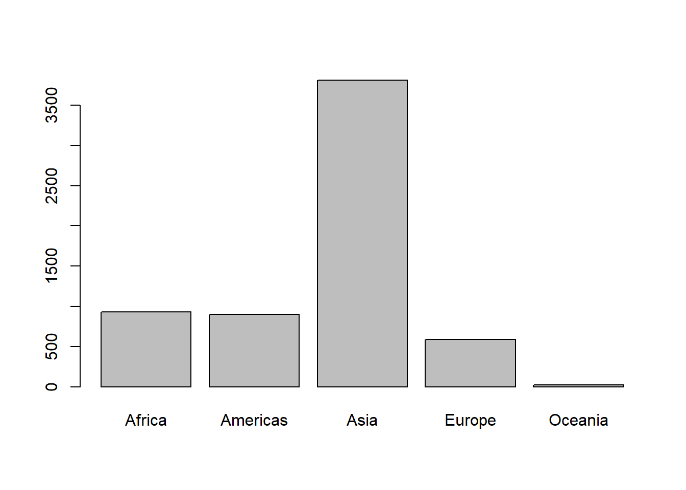
# reordering continent by population
pop_cont$continent <- fct_reorder(pop_cont$continent, pop_cont$pop, .desc = TRUE)
levels(pop_cont$continent)
#> [1] "Asia"     "Africa"   "Americas" "Europe"   "Oceania"

# sorting data frame by continent
pop_cont <- with(pop_cont, pop_cont[order(continent),])
pop_cont
#>   continent        pop
#> 3      Asia 3811953827
#> 1    Africa  929539692
#> 2  Americas  898871184
#> 4    Europe  586098529
#> 5   Oceania   24549947

# plotting barplot
with(pop_cont, barplot(pop/1e6, names.arg = continent))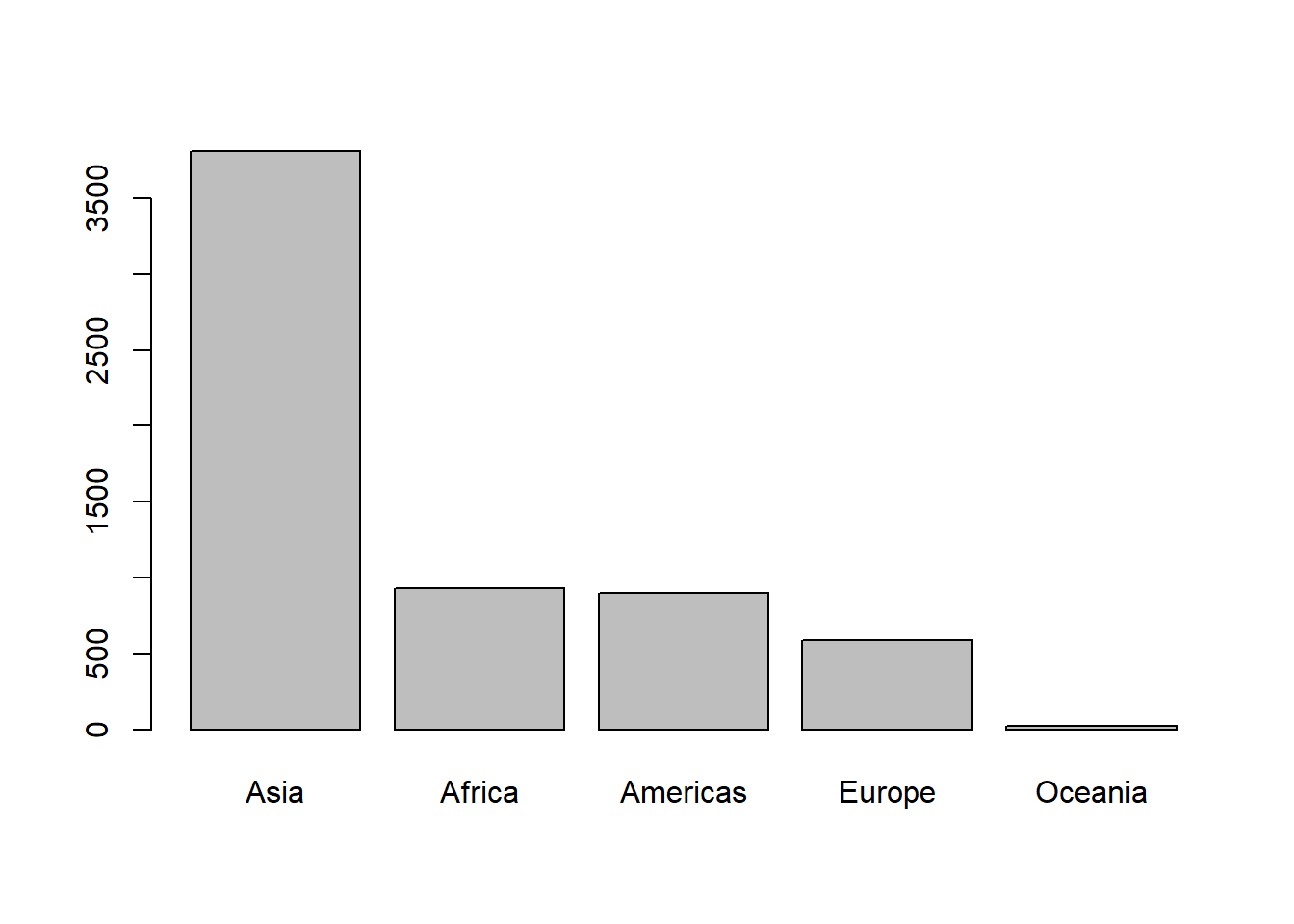
# producing an ascending bar chart
pop_cont$continent <- fct_reorder(pop_cont$continent, pop_cont$pop, .desc = FALSE)
pop_cont <- with(pop_cont, pop_cont[order(continent),])
with(pop_cont, barplot(pop/1e6, names.arg = continent))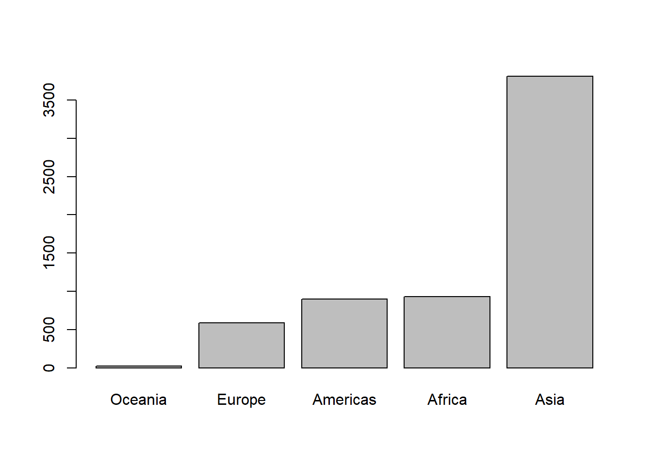
5.2.3 Restructuring levels and their labels
5.2.3.1 Renaming labels
The function fct_recode() is used to rename levels. It takes the form new_name = old_name.
levels(fct_recode(gapminder_2007$continent, 'AS' = 'Asia', 'Af' = 'Africa', 'Eu' = 'Europe'))
#> [1] "Americas" "Eu"       "Af"       "Oceania"  "AS"
5.2.3.2 collapsing levels
The function fct_collapse() is used to collapse levels into a new one.
# collapsing europe and africa into euroafrica
gapminder_2007$continent <-
  fct_collapse(gapminder_2007$continent, Euroafrica = c('Africa', 'Europe'))
table(gapminder_2007$continent)
#>
#>   Americas Euroafrica    Oceania       Asia
#>         25         82          2         33

# population by continent
(pop_cont <- aggregate(pop ~ continent, gapminder_2007, sum))
#>    continent        pop
#> 1   Americas  898871184
#> 2 Euroafrica 1515638221
#> 3    Oceania   24549947
#> 4       Asia 3811953827
5.2.3.3 combining levels
The functions fct_lump() and fct_lump_min() combines levels together based on the frequency of occurrence of each level.
# combining the least frequent levels
gapminder_2007 <- subset(gapminder, year == 2007, -3)
table(fct_lump(gapminder_2007$continent))
#>
#> Africa   Asia Europe  Other
#>     52     33     30     27
Using the arguments n= and p= we can specify the type of combining to perform; with positive values indicating combining rarest levels while negative values indicate combining most common levels.
# combining all except the first most common
table(fct_lump(gapminder_2007$continent, n = 1))
#>
#> Africa  Other
#>     52     90

# combining all except the first 2 most common
table(fct_lump(gapminder_2007$continent, n = 2))
#>
#> Africa   Asia  Other
#>     52     33     57

# combining all except the first 3 most common
table(fct_lump(gapminder_2007$continent, n = 3))
#>
#> Africa   Asia Europe  Other
#>     52     33     30     27

# combining all except the first rarest
table(fct_lump(gapminder_2007$continent, n = -1))
#>
#> Oceania   Other
#>       2     140

# combining all except the first 2 rarest
table(fct_lump(gapminder_2007$continent, n = -2))
#>
#> Americas  Oceania    Other
#>       25        2      115

# combining all except the first 3 rarest
table(fct_lump(gapminder_2007$continent, n = -3))
#>
#> Americas   Europe  Oceania    Other
#>       25       30        2       85

# using prop positive
table(fct_lump(gapminder_2007$continent, prop = 0.25))
#>
#> Africa  Other
#>     52     90
table(fct_lump(gapminder_2007$continent, prop = 0.22))
#>
#> Africa   Asia  Other
#>     52     33     57
table(fct_lump(gapminder_2007$continent, prop = 0.2))
#>
#> Africa   Asia Europe  Other
#>     52     33     30     27

# using prop negative
table(fct_lump(gapminder_2007$continent, prop = -0.25))
#>
#> Americas     Asia   Europe  Oceania    Other
#>       25       33       30        2       52
table(fct_lump(gapminder_2007$continent, prop = -0.22))
#>
#> Americas   Europe  Oceania    Other
#>       25       30        2       85
table(fct_lump(gapminder_2007$continent, prop = -0.2))
#>
#> Americas  Oceania    Other
#>       25        2      115
With fct_lump_min() combining is done based on whether a threshold declared by the min argument is met.
table(gapminder_2007$continent)
#>
#>   Africa Americas     Asia   Europe  Oceania
#>       52       25       33       30        2

# combining levels with less than 25 counts
table(fct_lump_min(gapminder_2007$continent, min = 25))
#>
#>   Africa Americas     Asia   Europe    Other
#>       52       25       33       30        2

# combining levels with less than 30 counts
table(fct_lump_min(gapminder_2007$continent, min = 30))
#>
#> Africa   Asia Europe  Other
#>     52     33     30     27

# combining levels with less than 33 counts
table(fct_lump_min(gapminder_2007$continent, min = 33))
#>
#> Africa   Asia  Other
#>     52     33     57
5.2.4 Remove and add levels
5.2.4.1 dropping levels
The function fct_other() will drop levels and replace them with the argument other_level = other by default.
# keeping asia and europe
table(fct_other(gapminder_2007$continent, keep = c('Asia', 'Europe')))
#>
#>   Asia Europe  Other
#>     33     30     79

# dropping asia and europe
table(fct_other(gapminder_2007$continent, drop = c('Asia', 'Europe')))
#>
#>   Africa Americas  Oceania    Other
#>       52       25        2       63

# replacing other continents with nonEurasia
table(fct_other(gapminder_2007$continent,
                keep = c('Asia', 'Europe'),
                other_level = 'nonEurasia'))
#>
#>       Asia     Europe nonEurasia
#>         33         30         79

# replacing europe and asia with Eurasia
table(fct_other(gapminder_2007$continent,
                drop = c('Asia', 'Europe'),
                other_level = 'Eurasia'))
#>
#>   Africa Americas  Oceania  Eurasia
#>       52       25        2       63
5.2.5 dropping unused levels
The function fct_drop() is used to drop unused levels. Unused levels are usually a problem while plotting as they appear on the graph though they contain no data.
# dropping Oceania
gapminder_oc <- subset(gapminder_2007, continent != 'Oceania')
table(gapminder_oc$continent)
#>
#>   Africa Americas     Asia   Europe  Oceania
#>       52       25       33       30        0
# Because the level Oceania has not been dropped, it appears on the above plot.
plot(gapminder_oc$continent)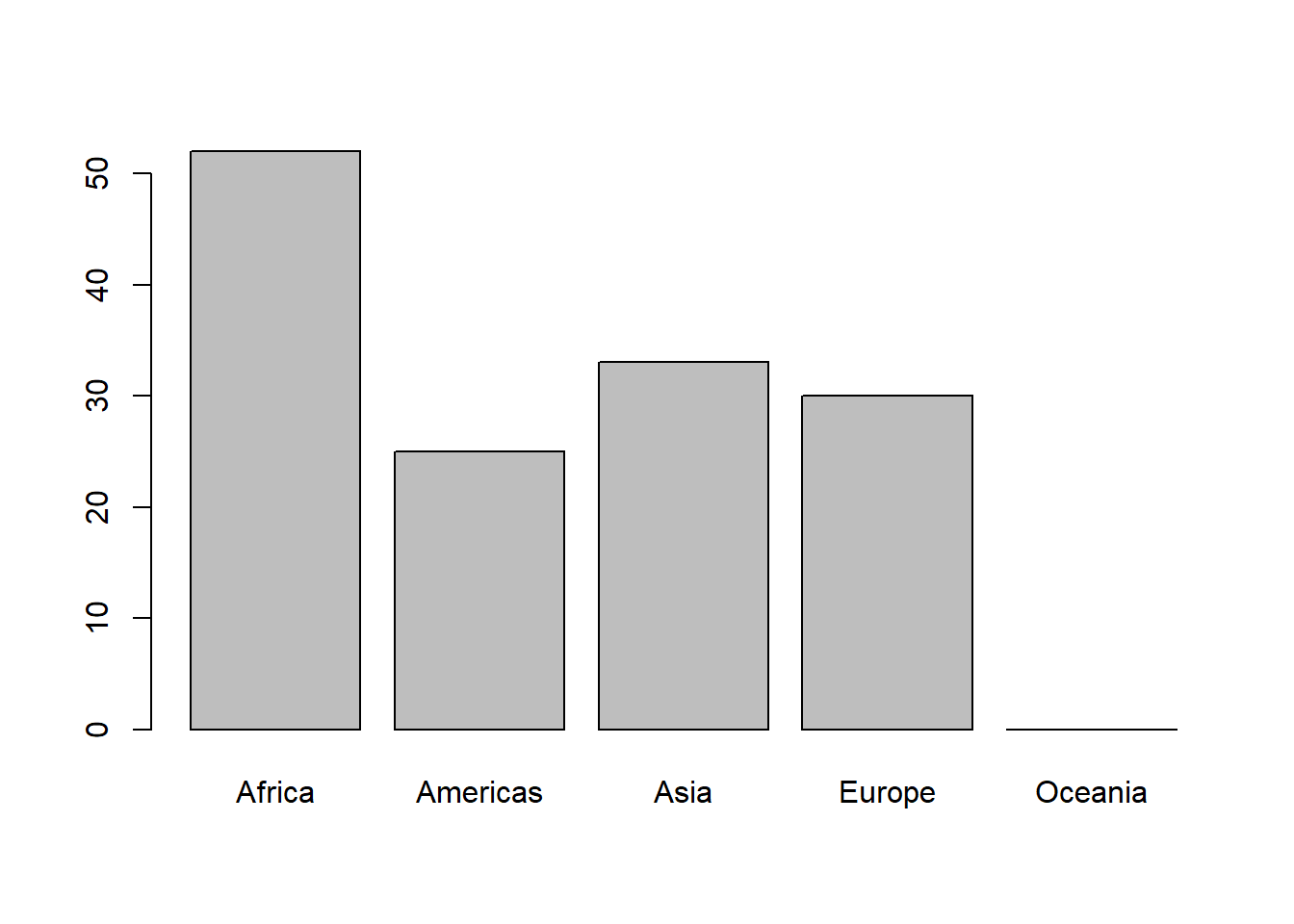
# dropping unused level
table(fct_drop(gapminder_oc$continent))
#>
#>   Africa Americas     Asia   Europe
#>       52       25       33       30
plot(fct_drop(gapminder_oc$continent))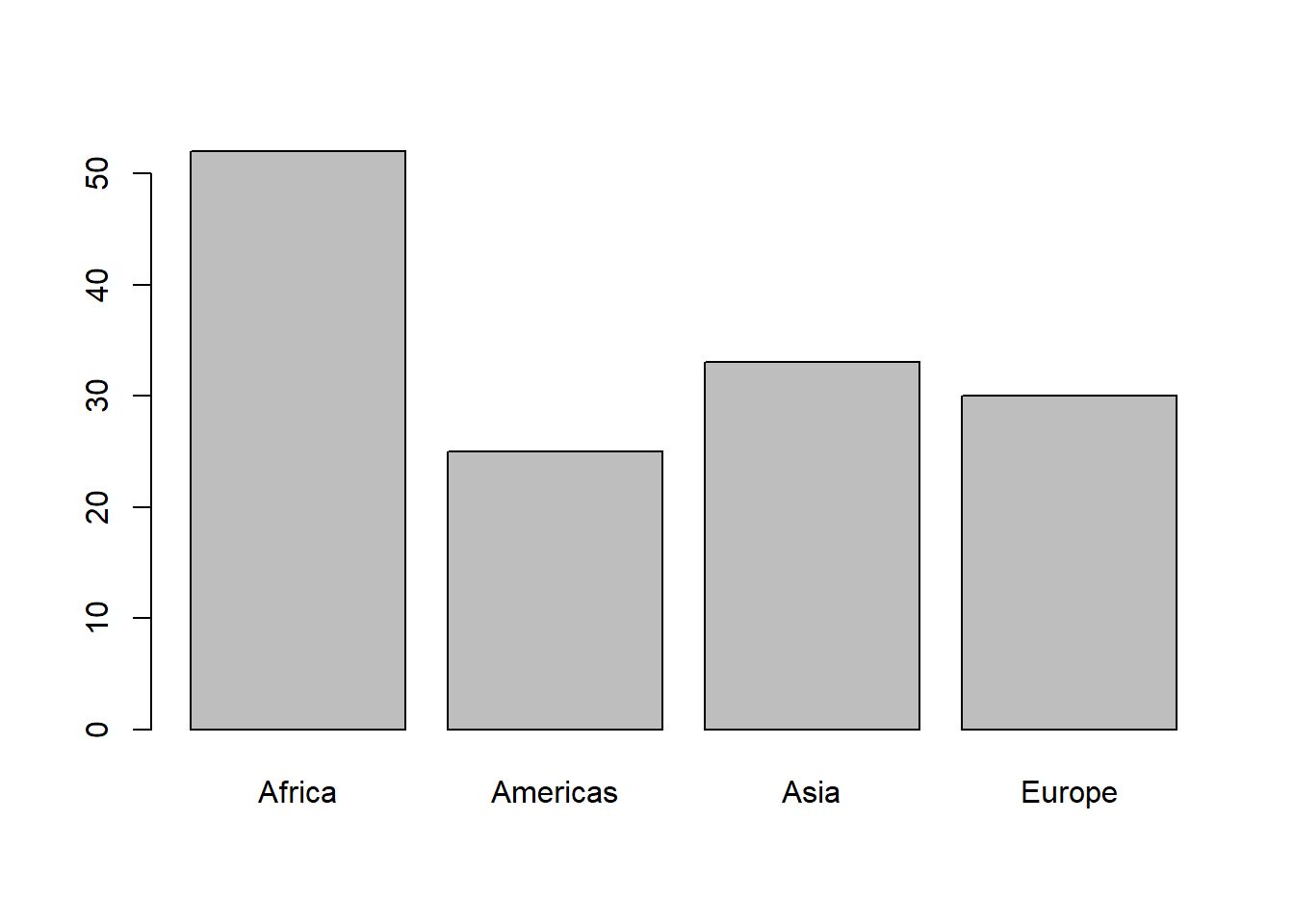
5.2.5.1 adding levels
The function fct_expand() is used to add levels.
# adding the level arctic
table(fct_expand(gapminder_oc$continent, 'arctic'))
#>
#>   Africa Americas     Asia   Europe  Oceania   arctic
#>       52       25       33       30        0        0

# adding the levels arctic and antarctica
table(fct_expand(gapminder_oc$continent, c('arctic', 'antarctica')))
#>
#>     Africa   Americas       Asia     Europe    Oceania
#>         52         25         33         30          0
#>     arctic antarctica
#>          0          0
# newly added levels appear on the plot though they have no data
plot(fct_expand(gapminder_oc$continent, c('arctic', 'antarctica')))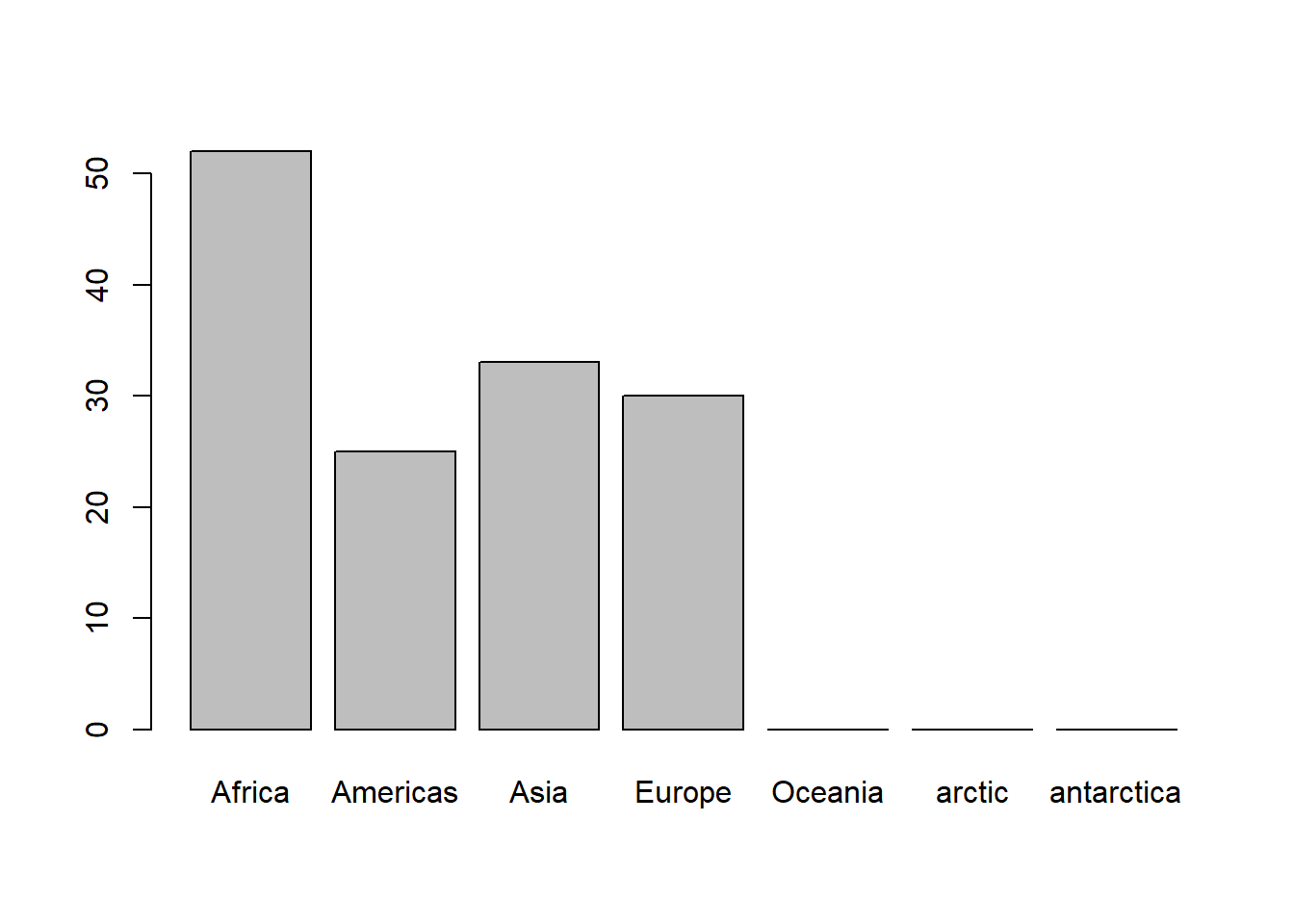
5.3 Data Manipulation with dplyr and tidyr
The package dplyr is one of the core packages in a group of packages known as the tidyverse. It was developed and released in 2014 by Hadley Wickham and others. dplyr is meant to be for data manipulation what ggplot2 is for data visualization, that is the grammar of data manipulation. It focuses solely on data frame manipulation and transformation using a set of verbs (functions) which are consistent and easy to understand.
Since dyplr belongs to the tidyverse world, it can be installed either by installing tidyverse or by installing dplyr itself.
5.3.1 Rename columns and rows
5.3.1.1 Renaming columns
The function rename() is used to rename columns.
library(readr)
library(dplyr)
library(gapminder)

# loading data
data(gapminder)
# get column names
names(gapminder)
#> [1] "country"   "continent" "year"      "lifeExp"
#> [5] "pop"       "gdpPercap"

# set column names
gapminder <- rename(gapminder,
                    Country = country,
                    Continent = continent,
                    Year = year,
                    `Life Expectancy` = lifeExp,
                    Population = pop,
                    `GDP per Capita` = gdpPercap)
# get column names
colnames(gapminder)
#> [1] "Country"         "Continent"       "Year"
#> [4] "Life Expectancy" "Population"      "GDP per Capita"
5.3.1.2 Renaming rows
Tibble does not support row names. See this.
5.3.2 Select columns and filter rows
5.3.2.1 Selecting and dropping columns
The function select() is used to select and rename columns.
# preparing data
column_names <- c('Rank', 'Title', 'Genre', 'Description', 'Director', 'Actors',
                  'Year', 'Runtime', 'Rating', 'Votes', 'Revenue', 'Metascore')
mov <- read.table(file = "data/IMDB-Movie-Data.csv", header = T, sep = ",", dec = ".", fileEncoding = "UTF-8", quote = "\"",
                  comment.char = "")
head(mov, 3)
#>   Rank                   Title                    Genre
#> 1    1 Guardians of the Galaxy  Action,Adventure,Sci-Fi
#> 2    2              Prometheus Adventure,Mystery,Sci-Fi
#> 3    3                   Split          Horror,Thriller
#>                                                                                                                                                     Description
#> 1                               A group of intergalactic criminals are forced to work together to stop a fanatical warrior from taking control of the universe.
#> 2                               Following clues to the origin of mankind, a team finds a structure on a distant moon, but they soon realize they are not alone.
#> 3 Three girls are kidnapped by a man with a diagnosed 23 distinct personalities. They must try to escape before the apparent emergence of a frightful new 24th.
#>             Director
#> 1         James Gunn
#> 2       Ridley Scott
#> 3 M. Night Shyamalan
#>                                                                    Actors
#> 1                    Chris Pratt, Vin Diesel, Bradley Cooper, Zoe Saldana
#> 2 Noomi Rapace, Logan Marshall-Green, Michael Fassbender, Charlize Theron
#> 3        James McAvoy, Anya Taylor-Joy, Haley Lu Richardson, Jessica Sula
#>   Year Runtime..Minutes. Rating  Votes Revenue..Millions.
#> 1 2014               121    8.1 757074             333.13
#> 2 2012               124    7.0 485820             126.46
#> 3 2016               117    7.3 157606             138.12
#>   Metascore
#> 1        76
#> 2        65
#> 3        62
names(mov) <- c('Rank', 'Title', 'Genre', 'Description', 'Director', 'Actors',
                  'Year', 'Runtime', 'Rating', 'Votes', 'Revenue', 'Metascore')


# selecting columns by column names
movies <- select(mov, c('Title', 'Year', 'Revenue', 'Metascore'))
head(movies, 3)
#>                     Title Year Revenue Metascore
#> 1 Guardians of the Galaxy 2014  333.13        76
#> 2              Prometheus 2012  126.46        65
#> 3                   Split 2016  138.12        62

# columns can be passed directly without quotation marks
movies <- select(mov, Title, Year, Revenue, Metascore)
head(movies, 3)
#>                     Title Year Revenue Metascore
#> 1 Guardians of the Galaxy 2014  333.13        76
#> 2              Prometheus 2012  126.46        65
#> 3                   Split 2016  138.12        62

# renaming column
movies <- select(mov,
                 Title,
                 `Release Year` = Year,
                 `Revenue in Millions` = Revenue,
                 Metascore)
head(movies, 3)
#>                     Title Release Year Revenue in Millions
#> 1 Guardians of the Galaxy         2014              333.13
#> 2              Prometheus         2012              126.46
#> 3                   Split         2016              138.12
#>   Metascore
#> 1        76
#> 2        65
#> 3        62

# selecting columns by position
movies <- select(mov, 2, 7, 11, 12)
head(movies, 3)
#>                     Title Year Revenue Metascore
#> 1 Guardians of the Galaxy 2014  333.13        76
#> 2              Prometheus 2012  126.46        65
#> 3                   Split 2016  138.12        62

# selecting columns by sequencing
movies <- select(mov, 7:12)
head(movies, 3)
#>   Year Runtime Rating  Votes Revenue Metascore
#> 1 2014     121    8.1 757074  333.13        76
#> 2 2012     124    7.0 485820  126.46        65
#> 3 2016     117    7.3 157606  138.12        62

# : works with column names
movies <- select(mov, Year:Metascore)
head(movies, 3)
#>   Year Runtime Rating  Votes Revenue Metascore
#> 1 2014     121    8.1 757074  333.13        76
#> 2 2012     124    7.0 485820  126.46        65
#> 3 2016     117    7.3 157606  138.12        62

# dropping columns by column names
movies <- select(mov, -Rank, -Genre, -Description,
                  -Director, -Actors, -Runtime, -Rating, -Votes)
head(movies, 3)
#>                     Title Year Revenue Metascore
#> 1 Guardians of the Galaxy 2014  333.13        76
#> 2              Prometheus 2012  126.46        65
#> 3                   Split 2016  138.12        62

# dropping columns by sequence
movies <- select(mov, -(1:6))
head(movies, 3)
#>   Year Runtime Rating  Votes Revenue Metascore
#> 1 2014     121    8.1 757074  333.13        76
#> 2 2012     124    7.0 485820  126.46        65
#> 3 2016     117    7.3 157606  138.12        62

movies <- select(mov, -(Rank:Actors))
head(movies, 3)
#>   Year Runtime Rating  Votes Revenue Metascore
#> 1 2014     121    8.1 757074  333.13        76
#> 2 2012     124    7.0 485820  126.46        65
#> 3 2016     117    7.3 157606  138.12        62

# dropping columns by index position
movies <- select(mov, -c(1, 3, 4, 5, 6, 8, 9, 10))
head(movies, 3)
#>                     Title Year Revenue Metascore
#> 1 Guardians of the Galaxy 2014  333.13        76
#> 2              Prometheus 2012  126.46        65
#> 3                   Split 2016  138.12        62

# dropping columns by index position
movies <- select(mov, -1, -3, -4, -5, -6, -8, -9, -10)
head(movies, 3)
#>                     Title Year Revenue Metascore
#> 1 Guardians of the Galaxy 2014  333.13        76
#> 2              Prometheus 2012  126.46        65
#> 3                   Split 2016  138.12        62
5.3.2.2 Selecting column based on a condition
The functions starts_with(), ends_with(), matches(), and contains() are used to select columns based on a specific pattern. The function
-
starts_with(): returns columns that start with a specific prefix -
ends_with(): returns columns that end with a specific suffix -
matches(): returns columns that match a particular regex pattern -
contains(): returns columns that contain a particular string
# selecting columns starting with R
movies <- select(mov, starts_with('R'))
head(movies, 3)
#>   Rank Runtime Rating Revenue
#> 1    1     121    8.1  333.13
#> 2    2     124    7.0  126.46
#> 3    3     117    7.3  138.12

# selecting columns starting with R and D
movies <- select(mov, starts_with(c('R', 'M')))
head(movies)
#>   Rank Runtime Rating Revenue Metascore
#> 1    1     121    8.1  333.13        76
#> 2    2     124    7.0  126.46        65
#> 3    3     117    7.3  138.12        62
#> 4    4     108    7.2  270.32        59
#> 5    5     123    6.2  325.02        40
#> 6    6     103    6.1   45.13        42

# selecting columns containing ea
movies <- select(mov, contains('ea'))
head(movies)
#>   Year
#> 1 2014
#> 2 2012
#> 3 2016
#> 4 2016
#> 5 2016
#> 6 2016

# selecting columns ending with r
movies <- select(mov, ends_with('r'))
head(movies)
#>               Director Year
#> 1           James Gunn 2014
#> 2         Ridley Scott 2012
#> 3   M. Night Shyamalan 2016
#> 4 Christophe Lourdelet 2016
#> 5           David Ayer 2016
#> 6          Yimou Zhang 2016

# selecting columns ending with r and e
movies <- select(mov, ends_with(c('k','r')))
head(movies)
#>   Rank             Director Year
#> 1    1           James Gunn 2014
#> 2    2         Ridley Scott 2012
#> 3    3   M. Night Shyamalan 2016
#> 4    4 Christophe Lourdelet 2016
#> 5    5           David Ayer 2016
#> 6    6          Yimou Zhang 2016
5.3.3 Selecting a single column
Selecting a single column with select() returns a one-column data frame. Often, a vector is wanted instead, to that end there is the function pull().
The function pull() is used to select a single column and return a vector.
movies <- select(mov, c('Title', 'Year', 'Revenue', 'Metascore'))

# using select returns a tibble
head(select(movies, 'Title'), 3)
#>                     Title
#> 1 Guardians of the Galaxy
#> 2              Prometheus
#> 3                   Split
class(select(movies, 'Title'))
#> [1] "data.frame"

# using pull returns a vector whose type depends on the data type of the column
head(pull(movies, var = 1))
#> [1] "Guardians of the Galaxy" "Prometheus"
#> [3] "Split"                   "Sing"
#> [5] "Suicide Squad"           "The Great Wall"
class(pull(movies, var = 1))
#> [1] "character"
5.3.4 Filtering rows
The function filter() is used to filter rows.
movies <- select(mov, -c(1, 3, 4, 6, 8, 10))

# using the filter() function
movies. <- filter(movies, Year == 2006)
head(movies., 3)
#>                                        Title
#> 1                               The Prestige
#> 2 Pirates of the Caribbean: Dead Man's Chest
#> 3                               The Departed
#>            Director Year Rating Revenue Metascore
#> 1 Christopher Nolan 2006    8.5   53.08        66
#> 2    Gore Verbinski 2006    7.3  423.03        53
#> 3   Martin Scorsese 2006    8.5  132.37        85
tail(movies., 3)
#>                                          Title
#> 42 Talladega Nights: The Ballad of Ricky Bobby
#> 43                         Lucky Number Slevin
#> 44                               Inland Empire
#>         Director Year Rating Revenue Metascore
#> 42    Adam McKay 2006    6.6  148.21        66
#> 43 Paul McGuigan 2006    7.8   22.49        53
#> 44   David Lynch 2006    7.0      NA        NA

# selecting movies released in 2006 with a rating above 8
filter(movies, Year == 2006 & Rating >= 8)
#>                      Title                         Director
#> 1             The Prestige                Christopher Nolan
#> 2             The Departed                  Martin Scorsese
#> 3            Casino Royale                  Martin Campbell
#> 4          Pan's Labyrinth               Guillermo del Toro
#> 5      The Lives of Others Florian Henckel von Donnersmarck
#> 6 The Pursuit of Happyness                 Gabriele Muccino
#> 7            Blood Diamond                     Edward Zwick
#>   Year Rating Revenue Metascore
#> 1 2006    8.5   53.08        66
#> 2 2006    8.5  132.37        85
#> 3 2006    8.0  167.01        80
#> 4 2006    8.2   37.62        98
#> 5 2006    8.5   11.28        89
#> 6 2006    8.0  162.59        64
#> 7 2006    8.0   57.37        64

# without the & operator
filter(movies, Year == 2006, Rating >= 8)
#>                      Title                         Director
#> 1             The Prestige                Christopher Nolan
#> 2             The Departed                  Martin Scorsese
#> 3            Casino Royale                  Martin Campbell
#> 4          Pan's Labyrinth               Guillermo del Toro
#> 5      The Lives of Others Florian Henckel von Donnersmarck
#> 6 The Pursuit of Happyness                 Gabriele Muccino
#> 7            Blood Diamond                     Edward Zwick
#>   Year Rating Revenue Metascore
#> 1 2006    8.5   53.08        66
#> 2 2006    8.5  132.37        85
#> 3 2006    8.0  167.01        80
#> 4 2006    8.2   37.62        98
#> 5 2006    8.5   11.28        89
#> 6 2006    8.0  162.59        64
#> 7 2006    8.0   57.37        64

# selecting rows with NA values on the Metascore column
movies. <- filter(movies, is.na(Metascore))
head(movies.)
#>                     Title             Director Year Rating
#> 1         Paris pieds nus       Dominique Abel 2016    6.8
#> 2 Bahubali: The Beginning       S.S. Rajamouli 2015    8.3
#> 3              Dead Awake       Phillip Guzman 2016    4.7
#> 4               5- 25- 77 Patrick Read Johnson 2007    7.1
#> 5 Don't Fuck in the Woods        Shawn Burkett 2016    2.7
#> 6                  Fallen          Scott Hicks 2016    5.6
#>   Revenue Metascore
#> 1      NA        NA
#> 2    6.50        NA
#> 3    0.01        NA
#> 4      NA        NA
#> 5      NA        NA
#> 6      NA        NA

# selecting rows with NA values on the Revenue and Metascore column
movies. <- filter(movies, is.na(Revenue), is.na(Metascore))
head(movies.)
#>                     Title             Director Year Rating
#> 1         Paris pieds nus       Dominique Abel 2016    6.8
#> 2               5- 25- 77 Patrick Read Johnson 2007    7.1
#> 3 Don't Fuck in the Woods        Shawn Burkett 2016    2.7
#> 4                  Fallen          Scott Hicks 2016    5.6
#> 5            Contratiempo          Oriol Paulo 2016    7.9
#> 6    Boyka: Undisputed IV      Todor Chapkanov 2016    7.4
#>   Revenue Metascore
#> 1      NA        NA
#> 2      NA        NA
#> 3      NA        NA
#> 4      NA        NA
#> 5      NA        NA
#> 6      NA        NA

# selecting rows with NA values on either the Revenue or Metascore column
movies. <- filter(movies, is.na(Revenue) | is.na(Metascore))
head(movies.)
#>                     Title             Director Year Rating
#> 1                Mindhorn           Sean Foley 2016    6.4
#> 2          Hounds of Love            Ben Young 2016    6.7
#> 3         Paris pieds nus       Dominique Abel 2016    6.8
#> 4 Bahubali: The Beginning       S.S. Rajamouli 2015    8.3
#> 5              Dead Awake       Phillip Guzman 2016    4.7
#> 6               5- 25- 77 Patrick Read Johnson 2007    7.1
#>   Revenue Metascore
#> 1      NA        71
#> 2      NA        72
#> 3      NA        NA
#> 4    6.50        NA
#> 5    0.01        NA
#> 6      NA        NA

# selecting rows without NA values on the Metascore column
movies. <- filter(movies, !is.na(Metascore))
head(movies.)
#>                     Title             Director Year Rating
#> 1 Guardians of the Galaxy           James Gunn 2014    8.1
#> 2              Prometheus         Ridley Scott 2012    7.0
#> 3                   Split   M. Night Shyamalan 2016    7.3
#> 4                    Sing Christophe Lourdelet 2016    7.2
#> 5           Suicide Squad           David Ayer 2016    6.2
#> 6          The Great Wall          Yimou Zhang 2016    6.1
#>   Revenue Metascore
#> 1  333.13        76
#> 2  126.46        65
#> 3  138.12        62
#> 4  270.32        59
#> 5  325.02        40
#> 6   45.13        42

# selecting rows without NA values on the Revenue and Metascore columns
movies. <- filter(movies, !is.na(Revenue), !is.na(Metascore))
head(movies.)
#>                     Title             Director Year Rating
#> 1 Guardians of the Galaxy           James Gunn 2014    8.1
#> 2              Prometheus         Ridley Scott 2012    7.0
#> 3                   Split   M. Night Shyamalan 2016    7.3
#> 4                    Sing Christophe Lourdelet 2016    7.2
#> 5           Suicide Squad           David Ayer 2016    6.2
#> 6          The Great Wall          Yimou Zhang 2016    6.1
#>   Revenue Metascore
#> 1  333.13        76
#> 2  126.46        65
#> 3  138.12        62
#> 4  270.32        59
#> 5  325.02        40
#> 6   45.13        42
nrow(movies.)
#> [1] 838

# selecting rows without NA values on either the Revenue or Metascore columns
movies. <- filter(movies, !is.na(Revenue) | !is.na(Metascore))
head(movies.)
#>                     Title             Director Year Rating
#> 1 Guardians of the Galaxy           James Gunn 2014    8.1
#> 2              Prometheus         Ridley Scott 2012    7.0
#> 3                   Split   M. Night Shyamalan 2016    7.3
#> 4                    Sing Christophe Lourdelet 2016    7.2
#> 5           Suicide Squad           David Ayer 2016    6.2
#> 6          The Great Wall          Yimou Zhang 2016    6.1
#>   Revenue Metascore
#> 1  333.13        76
#> 2  126.46        65
#> 3  138.12        62
#> 4  270.32        59
#> 5  325.02        40
#> 6   45.13        42

nrow(movies.)
#> [1] 970

# selecting films released in 2006 and 2008
movies. <- filter(movies, Year %in% c(2006, 2008))
head(movies.)
#>                                        Title
#> 1                            The Dark Knight
#> 2                               The Prestige
#> 3 Pirates of the Caribbean: Dead Man's Chest
#> 4                               The Departed
#> 5                                        300
#> 6                                 Mamma Mia!
#>            Director Year Rating Revenue Metascore
#> 1 Christopher Nolan 2008    9.0  533.32        82
#> 2 Christopher Nolan 2006    8.5   53.08        66
#> 3    Gore Verbinski 2006    7.3  423.03        53
#> 4   Martin Scorsese 2006    8.5  132.37        85
#> 5       Zack Snyder 2006    7.7  210.59        52
#> 6    Phyllida Lloyd 2008    6.4  143.70        51

# selecting films released by 'James Gunn' or 'James Marsh'
movies. <- filter(movies, Director %in% c('James Gunn', 'James Marsh'))
head(movies.)
#>                      Title    Director Year Rating Revenue
#> 1  Guardians of the Galaxy  James Gunn 2014    8.1  333.13
#> 2 The Theory of Everything James Marsh 2014    7.7   35.89
#> 3                  Slither  James Gunn 2006    6.5    7.77
#> 4                    Super  James Gunn 2010    6.8    0.32
#>   Metascore
#> 1        76
#> 2        72
#> 3        69
#> 4        50

# selecting films released between 2006 and 2008
movies. <- filter(movies, between(Year, 2006, 2008))
head(movies., 3)
#>             Title             Director Year Rating Revenue
#> 1       5- 25- 77 Patrick Read Johnson 2007    7.1      NA
#> 2 The Dark Knight    Christopher Nolan 2008    9.0  533.32
#> 3    The Prestige    Christopher Nolan 2006    8.5   53.08
#>   Metascore
#> 1        NA
#> 2        82
#> 3        66
tail(movies., 3)
#>                      Title   Director Year Rating Revenue
#> 147       Taare Zameen Par Aamir Khan 2007    8.5    1.20
#> 148        Hostel: Part II   Eli Roth 2007    5.5   17.54
#> 149 Step Up 2: The Streets Jon M. Chu 2008    6.2   58.01
#>     Metascore
#> 147        42
#> 148        46
#> 149        50
5.3.4.1 Randomly selecting rows
The function sample_frac() randomly samples rows and returns a fixed fraction of them.
# sampling by a proportion
sample_frac(movies, 0.005, replace = TRUE)
#>               Title       Director Year Rating Revenue
#> 1          Bad Moms      Jon Lucas 2016    6.2  113.08
#> 2       Rescue Dawn  Werner Herzog 2006    7.3    5.48
#> 3       Rescue Dawn  Werner Herzog 2006    7.3    5.48
#> 4 The Warriors Gate Matthias Hoene 2016    5.3      NA
#> 5  Marie Antoinette  Sofia Coppola 2006    6.4   15.96
#>   Metascore
#> 1        60
#> 2        77
#> 3        77
#> 4        77
#> 5        65
The function sample_n() randomly samples rows and returns a fixed number of them.
# sampling by number
sample_n(movies, 5, replace = TRUE)
#>                  Title         Director Year Rating Revenue
#> 1                Youth Paolo Sorrentino 2015    7.3    2.70
#> 2            Brimstone Martin Koolhoven 2016    7.1      NA
#> 3 Perfetti sconosciuti   Paolo Genovese 2016    7.7      NA
#> 4             Watchmen      Zack Snyder 2009    7.6  107.50
#> 5            Footloose     Craig Brewer 2011    5.9   51.78
#>   Metascore
#> 1        64
#> 2        44
#> 3        43
#> 4        56
#> 5        58
5.3.5 Slicing
The function slice() is used to slice a data set.
slice(movies, 200:205)
#>                  Title                Director Year Rating
#> 1 Central Intelligence Rawson Marshall Thurber 2016    6.3
#> 2     Edge of Tomorrow              Doug Liman 2014    7.9
#> 3  A Cure for Wellness          Gore Verbinski 2016    6.5
#> 4              Snowden            Oliver Stone 2016    7.3
#> 5             Iron Man             Jon Favreau 2008    7.9
#> 6            Allegiant        Robert Schwentke 2016    5.7
#>   Revenue Metascore
#> 1  127.38        52
#> 2  100.19        71
#> 3    8.10        47
#> 4   21.48        58
#> 5  318.30        79
#> 6   66.00        33
5.3.6 Top values
The function top_n() returns the top nth number of elements in a column.
# top 5 movies by revenue
top_n(movies, 5, Revenue)
#>                                        Title
#> 1 Star Wars: Episode VII - The Force Awakens
#> 2                            The Dark Knight
#> 3                               The Avengers
#> 4                             Jurassic World
#> 5                                     Avatar
#>            Director Year Rating Revenue Metascore
#> 1       J.J. Abrams 2015    8.1  936.63        81
#> 2 Christopher Nolan 2008    9.0  533.32        82
#> 3       Joss Whedon 2012    8.1  623.28        69
#> 4   Colin Trevorrow 2015    7.0  652.18        59
#> 5     James Cameron 2009    7.8  760.51        83

# if no column is specified, the last is used.
top_n(movies, 5)
#>                   Title           Director Year Rating
#> 1 Manchester by the Sea   Kenneth Lonergan 2016    7.9
#> 2             Moonlight      Barry Jenkins 2016    7.5
#> 3      12 Years a Slave      Steve McQueen 2013    8.1
#> 4       Pan's Labyrinth Guillermo del Toro 2006    8.2
#> 5           Ratatouille          Brad Bird 2007    8.0
#> 6               Gravity     Alfonso Cuarón 2013    7.8
#> 7               Boyhood  Richard Linklater 2014    7.9
#>   Revenue Metascore
#> 1   47.70        96
#> 2   27.85        99
#> 3   56.67        96
#> 4   37.62        98
#> 5  206.44        96
#> 6  274.08        96
#> 7   25.36       100
The function top_frac() returns the top nth elements in a column by proportion.
# top 0.5% of movies by revenue
top_frac(movies, 0.005, Revenue)
#>                                        Title
#> 1 Star Wars: Episode VII - The Force Awakens
#> 2                            The Dark Knight
#> 3                               The Avengers
#> 4                             Jurassic World
#> 5                                     Avatar
#>            Director Year Rating Revenue Metascore
#> 1       J.J. Abrams 2015    8.1  936.63        81
#> 2 Christopher Nolan 2008    9.0  533.32        82
#> 3       Joss Whedon 2012    8.1  623.28        69
#> 4   Colin Trevorrow 2015    7.0  652.18        59
#> 5     James Cameron 2009    7.8  760.51        83

# if no column is specified, the last is used.
top_frac(movies, 0.005)
#>                   Title           Director Year Rating
#> 1 Manchester by the Sea   Kenneth Lonergan 2016    7.9
#> 2             Moonlight      Barry Jenkins 2016    7.5
#> 3      12 Years a Slave      Steve McQueen 2013    8.1
#> 4       Pan's Labyrinth Guillermo del Toro 2006    8.2
#> 5           Ratatouille          Brad Bird 2007    8.0
#> 6               Gravity     Alfonso Cuarón 2013    7.8
#> 7               Boyhood  Richard Linklater 2014    7.9
#>   Revenue Metascore
#> 1   47.70        96
#> 2   27.85        99
#> 3   56.67        96
#> 4   37.62        98
#> 5  206.44        96
#> 6  274.08        96
#> 7   25.36       100
5.3.7 Using select and filter
select(filter(mov, Year == 2006, Rating >= 8), 2, 7, 9, 11, 12)
#>                      Title Year Rating Revenue Metascore
#> 1             The Prestige 2006    8.5   53.08        66
#> 2             The Departed 2006    8.5  132.37        85
#> 3            Casino Royale 2006    8.0  167.01        80
#> 4          Pan's Labyrinth 2006    8.2   37.62        98
#> 5      The Lives of Others 2006    8.5   11.28        89
#> 6 The Pursuit of Happyness 2006    8.0  162.59        64
#> 7            Blood Diamond 2006    8.0   57.37        64
filter(select(mov, 2, 7, 9, 11, 12), Year == 2006, Rating >= 8)
#>                      Title Year Rating Revenue Metascore
#> 1             The Prestige 2006    8.5   53.08        66
#> 2             The Departed 2006    8.5  132.37        85
#> 3            Casino Royale 2006    8.0  167.01        80
#> 4          Pan's Labyrinth 2006    8.2   37.62        98
#> 5      The Lives of Others 2006    8.5   11.28        89
#> 6 The Pursuit of Happyness 2006    8.0  162.59        64
#> 7            Blood Diamond 2006    8.0   57.37        64
With such an operation, it is better to use the pipe operator.
5.3.8 Pipe operator
The pipe operator (%>%) passes an object forward into a function. The shortcut Ctrl + Shift + M for PC and Cmd + Shift + M for Mac is used to insert this operator. Below, we pass the dataset mov into the function filter(), which after processing, passes its output to select().
# passing movies dataset into filter and then to select
mov %>%
  filter(Year == 2006 & Rating >= 8) %>%
  select(2, 7, 9, 11, 12)
#>                      Title Year Rating Revenue Metascore
#> 1             The Prestige 2006    8.5   53.08        66
#> 2             The Departed 2006    8.5  132.37        85
#> 3            Casino Royale 2006    8.0  167.01        80
#> 4          Pan's Labyrinth 2006    8.2   37.62        98
#> 5      The Lives of Others 2006    8.5   11.28        89
#> 6 The Pursuit of Happyness 2006    8.0  162.59        64
#> 7            Blood Diamond 2006    8.0   57.37        64

mov %>%
  select(2, 7, 9, 11, 12) %>%
  filter(Year == 2006 & Rating >= 8)
#>                      Title Year Rating Revenue Metascore
#> 1             The Prestige 2006    8.5   53.08        66
#> 2             The Departed 2006    8.5  132.37        85
#> 3            Casino Royale 2006    8.0  167.01        80
#> 4          Pan's Labyrinth 2006    8.2   37.62        98
#> 5      The Lives of Others 2006    8.5   11.28        89
#> 6 The Pursuit of Happyness 2006    8.0  162.59        64
#> 7            Blood Diamond 2006    8.0   57.37        64
Using . as a placeholder for the data set. The period will be replaced in the function by the data frame or tibble.
mov %>%
  filter(.$Year == 2006 & .$Rating >= 8) %>%
  select(2, 7, 9, 11, 12)
#>                      Title Year Rating Revenue Metascore
#> 1             The Prestige 2006    8.5   53.08        66
#> 2             The Departed 2006    8.5  132.37        85
#> 3            Casino Royale 2006    8.0  167.01        80
#> 4          Pan's Labyrinth 2006    8.2   37.62        98
#> 5      The Lives of Others 2006    8.5   11.28        89
#> 6 The Pursuit of Happyness 2006    8.0  162.59        64
#> 7            Blood Diamond 2006    8.0   57.37        64
5.4 Manipulating Columns
5.4.1 Inserting a new column
The function mutate() and transmutate are used to manipulate columns. They are used to:
- insert new columns
- duplicate columns
- deriving new columns
- update existing ones
# adding a new column known as example
select(mov, c('Title', 'Year', 'Revenue', 'Metascore')) %>%
mutate(example = sample(1000)) %>%
  head()
#>                     Title Year Revenue Metascore example
#> 1 Guardians of the Galaxy 2014  333.13        76     459
#> 2              Prometheus 2012  126.46        65       4
#> 3                   Split 2016  138.12        62     130
#> 4                    Sing 2016  270.32        59     820
#> 5           Suicide Squad 2016  325.02        40     275
#> 6          The Great Wall 2016   45.13        42     153

# duplicating the Revenue column
select(mov, c('Title', 'Year', 'Revenue', 'Metascore')) %>%
mutate(Metascore.2 = Metascore) %>%
  head()
#>                     Title Year Revenue Metascore
#> 1 Guardians of the Galaxy 2014  333.13        76
#> 2              Prometheus 2012  126.46        65
#> 3                   Split 2016  138.12        62
#> 4                    Sing 2016  270.32        59
#> 5           Suicide Squad 2016  325.02        40
#> 6          The Great Wall 2016   45.13        42
#>   Metascore.2
#> 1          76
#> 2          65
#> 3          62
#> 4          59
#> 5          40
#> 6          42

# deriving the new column Movie Class
labels <- c('Very Low', 'Low', 'Moderate', 'High', 'Very High')

select(mov, c('Title', 'Year', 'Rating', 'Revenue', 'Metascore')) %>%
  mutate(`Movie Class` = cut(Rating, breaks = c(0, 5.5, 6.5, 7, 7.5, 10),
                           labels = labels)) %>%
  head()
#>                     Title Year Rating Revenue Metascore
#> 1 Guardians of the Galaxy 2014    8.1  333.13        76
#> 2              Prometheus 2012    7.0  126.46        65
#> 3                   Split 2016    7.3  138.12        62
#> 4                    Sing 2016    7.2  270.32        59
#> 5           Suicide Squad 2016    6.2  325.02        40
#> 6          The Great Wall 2016    6.1   45.13        42
#>   Movie Class
#> 1   Very High
#> 2    Moderate
#> 3        High
#> 4        High
#> 5         Low
#> 6         Low

# Updating the Director column to uppercase
select(mov, c(Title, Director, Year, Rating, Revenue, Metascore)) %>%
  mutate(Director = toupper(Director)) %>%
  head()
#>                     Title             Director Year Rating
#> 1 Guardians of the Galaxy           JAMES GUNN 2014    8.1
#> 2              Prometheus         RIDLEY SCOTT 2012    7.0
#> 3                   Split   M. NIGHT SHYAMALAN 2016    7.3
#> 4                    Sing CHRISTOPHE LOURDELET 2016    7.2
#> 5           Suicide Squad           DAVID AYER 2016    6.2
#> 6          The Great Wall          YIMOU ZHANG 2016    6.1
#>   Revenue Metascore
#> 1  333.13        76
#> 2  126.46        65
#> 3  138.12        62
#> 4  270.32        59
#> 5  325.02        40
#> 6   45.13        42

# using a customized function
# defining a function
fin_crisis <- function(x) {
    if(x < 2008){
        return('pre financial crisis')
    }else if(x < 2010 ){
        return('financial crisis')
    }else{
        return('post financial crisis')
    }
}

select(mov, 2, 7, 11, 12) %>%
  mutate('fin crisis Class' = sapply(Year, fin_crisis)) %>%
  head()
#>                     Title Year Revenue Metascore
#> 1 Guardians of the Galaxy 2014  333.13        76
#> 2              Prometheus 2012  126.46        65
#> 3                   Split 2016  138.12        62
#> 4                    Sing 2016  270.32        59
#> 5           Suicide Squad 2016  325.02        40
#> 6          The Great Wall 2016   45.13        42
#>        fin crisis Class
#> 1 post financial crisis
#> 2 post financial crisis
#> 3 post financial crisis
#> 4 post financial crisis
#> 5 post financial crisis
#> 6 post financial crisis

# deriving a new column from a calculation
select(mov, 2, 5, 7, 8, 11) %>%
  mutate('Rev/Run' = round(Revenue/Runtime, 2)) %>%
  head()
#>                     Title             Director Year Runtime
#> 1 Guardians of the Galaxy           James Gunn 2014     121
#> 2              Prometheus         Ridley Scott 2012     124
#> 3                   Split   M. Night Shyamalan 2016     117
#> 4                    Sing Christophe Lourdelet 2016     108
#> 5           Suicide Squad           David Ayer 2016     123
#> 6          The Great Wall          Yimou Zhang 2016     103
#>   Revenue Rev/Run
#> 1  333.13    2.75
#> 2  126.46    1.02
#> 3  138.12    1.18
#> 4  270.32    2.50
#> 5  325.02    2.64
#> 6   45.13    0.44
The function case_when() is a condensed form of if else statement or CASE THEN in SQL.
# classifying movies by ratings
select(mov, 2, 7, 9, 11, 12) %>%
  mutate(category = case_when(Rating < 5.5 ~ 'Very Low',
                              Rating < 6.5 ~ 'Low',
                              Rating < 7 ~ 'Moderate',
                              Rating < 7.5 ~ 'High',
                              Rating <= 10 ~ 'Very High')) %>%
  head()
#>                     Title Year Rating Revenue Metascore
#> 1 Guardians of the Galaxy 2014    8.1  333.13        76
#> 2              Prometheus 2012    7.0  126.46        65
#> 3                   Split 2016    7.3  138.12        62
#> 4                    Sing 2016    7.2  270.32        59
#> 5           Suicide Squad 2016    6.2  325.02        40
#> 6          The Great Wall 2016    6.1   45.13        42
#>    category
#> 1 Very High
#> 2      High
#> 3      High
#> 4      High
#> 5       Low
#> 6       Low
The function coalesce() which is modelled after the COALESCE function in SQL returns the first non-missing element. Using it, we can replace NA values in a column.
# selecting some rows containing NA values
select(mov, 2, 5, 7, 9, 11, 12) %>%
  filter(is.na(Revenue)) %>%
  slice(c(8, 23, 26, 40, 43, 48))
#>                      Title        Director Year Rating
#> 1  The Autopsy of Jane Doe   André Ovredal 2016    6.8
#> 2                  Old Boy       Spike Lee 2013    5.8
#> 3                  Satanic Jeffrey G. Hunt 2016    3.7
#> 4      Absolutely Anything     Terry Jones 2015    6.0
#> 5 The Headhunter's Calling   Mark Williams 2016    6.9
#> 6           Predestination Michael Spierig 2014    7.5
#>   Revenue Metascore
#> 1      NA        65
#> 2      NA        49
#> 3      NA        NA
#> 4      NA        31
#> 5      NA        85
#> 6      NA        69

# replacing NA values with a value
select(mov, 2, 5, 7, 9, 11, 12) %>%
  mutate(Revenue = coalesce(Revenue, 50)) %>%
  slice(c(8, 23, 26, 40, 43, 48))
#>                     Title             Director Year Rating
#> 1                Mindhorn           Sean Foley 2016    6.4
#> 2          Hounds of Love            Ben Young 2016    6.7
#> 3         Paris pieds nus       Dominique Abel 2016    6.8
#> 4               5- 25- 77 Patrick Read Johnson 2007    7.1
#> 5 Don't Fuck in the Woods        Shawn Burkett 2016    2.7
#> 6                  Fallen          Scott Hicks 2016    5.6
#>   Revenue Metascore
#> 1      50        71
#> 2      50        72
#> 3      50        NA
#> 4      50        NA
#> 5      50        NA
#> 6      50        NA

# replacing NA values with a computed value (mean/median)
select(mov, 2, 5, 7, 9, 11, 12) %>%
  mutate(Revenue = coalesce(Revenue, round(median(Revenue, na.rm = T))),
         Metascore = coalesce(Metascore, round(mean(Metascore, na.rm = T)))) %>%
  slice(c(8, 23, 26, 40, 43, 48))
#>                     Title             Director Year Rating
#> 1                Mindhorn           Sean Foley 2016    6.4
#> 2          Hounds of Love            Ben Young 2016    6.7
#> 3         Paris pieds nus       Dominique Abel 2016    6.8
#> 4               5- 25- 77 Patrick Read Johnson 2007    7.1
#> 5 Don't Fuck in the Woods        Shawn Burkett 2016    2.7
#> 6                  Fallen          Scott Hicks 2016    5.6
#>   Revenue Metascore
#> 1      48        71
#> 2      48        72
#> 3      48        59
#> 4      48        59
#> 5      48        59
#> 6      48        59
The function transmutate() behaves like mutate() but drops other columns that are not selected.
# transmutate drops unselected columns
select(mov, c(Title, Director, Year, Rating, Revenue, Metascore)) %>%
  transmute(Director = toupper(Director)) %>%
  head()
#>               Director
#> 1           JAMES GUNN
#> 2         RIDLEY SCOTT
#> 3   M. NIGHT SHYAMALAN
#> 4 CHRISTOPHE LOURDELET
#> 5           DAVID AYER
#> 6          YIMOU ZHANG

# transmutate keeps selected columns
select(mov, c(Title, Director, Year, Runtime, Revenue, Metascore)) %>%
  transmute(Director = toupper(Director),
            Year,
            Revenue = round(Revenue/Runtime, 2)) %>%
head()
#>               Director Year Revenue
#> 1           JAMES GUNN 2014    2.75
#> 2         RIDLEY SCOTT 2012    1.02
#> 3   M. NIGHT SHYAMALAN 2016    1.18
#> 4 CHRISTOPHE LOURDELET 2016    2.50
#> 5           DAVID AYER 2016    2.64
#> 6          YIMOU ZHANG 2016    0.44
5.5 Sorting and ranking
5.5.1 Sorting
The function arrange() is used to sort data frames. It does an ascending sort but to do a descending sort, we use the function desc() or the negative sign.
# sort increasing
select(mov, c(Title, Year, Runtime, Revenue, Metascore)) %>%
  arrange(Revenue) %>%
  head(10)
#>                       Title Year Runtime Revenue Metascore
#> 1          A Kind of Murder 2016      95    0.00        50
#> 2                Dead Awake 2016      99    0.01        NA
#> 3                 Wakefield 2016     106    0.01        61
#> 4                  Lovesong 2016      84    0.01        74
#> 5               Love, Rosie 2014     102    0.01        44
#> 6           Into the Forest 2015     101    0.01        59
#> 7                Stake Land 2010      98    0.02        66
#> 8            The First Time 2012      95    0.02        55
#> 9  The Blackcoat's Daughter 2015      93    0.02        68
#> 10         The Sea of Trees 2015     110    0.02        23

# sort decreasing using the negative sign
select(mov, c(Title, Year, Runtime, Revenue, Metascore)) %>%
  arrange(-Revenue) %>%
  head(10)
#>                                         Title Year Runtime
#> 1  Star Wars: Episode VII - The Force Awakens 2015     136
#> 2                                      Avatar 2009     162
#> 3                              Jurassic World 2015     124
#> 4                                The Avengers 2012     143
#> 5                             The Dark Knight 2008     152
#> 6                                   Rogue One 2016     133
#> 7                                Finding Dory 2016      97
#> 8                     Avengers: Age of Ultron 2015     141
#> 9                       The Dark Knight Rises 2012     164
#> 10            The Hunger Games: Catching Fire 2013     146
#>    Revenue Metascore
#> 1   936.63        81
#> 2   760.51        83
#> 3   652.18        59
#> 4   623.28        69
#> 5   533.32        82
#> 6   532.17        65
#> 7   486.29        77
#> 8   458.99        66
#> 9   448.13        78
#> 10  424.65        76

# sort decreasing using desc()
select(mov, c(Title, Year, Runtime, Revenue, Metascore)) %>%
  arrange(desc(Revenue)) %>%
  head(10)
#>                                         Title Year Runtime
#> 1  Star Wars: Episode VII - The Force Awakens 2015     136
#> 2                                      Avatar 2009     162
#> 3                              Jurassic World 2015     124
#> 4                                The Avengers 2012     143
#> 5                             The Dark Knight 2008     152
#> 6                                   Rogue One 2016     133
#> 7                                Finding Dory 2016      97
#> 8                     Avengers: Age of Ultron 2015     141
#> 9                       The Dark Knight Rises 2012     164
#> 10            The Hunger Games: Catching Fire 2013     146
#>    Revenue Metascore
#> 1   936.63        81
#> 2   760.51        83
#> 3   652.18        59
#> 4   623.28        69
#> 5   533.32        82
#> 6   532.17        65
#> 7   486.29        77
#> 8   458.99        66
#> 9   448.13        78
#> 10  424.65        76


# sorting on multiple columns
select(mov, c(Title, Year, Runtime, Revenue, Metascore)) %>%
  arrange(-Metascore, Revenue) %>%
  head(10)
#>                    Title Year Runtime Revenue Metascore
#> 1                Boyhood 2014     165   25.36       100
#> 2              Moonlight 2016     111   27.85        99
#> 3        Pan's Labyrinth 2006     118   37.62        98
#> 4  Manchester by the Sea 2016     137   47.70        96
#> 5       12 Years a Slave 2013     134   56.67        96
#> 6            Ratatouille 2007     111  206.44        96
#> 7                Gravity 2013      91  274.08        96
#> 8                  Carol 2015     118    0.25        95
#> 9       Zero Dark Thirty 2012     157   95.72        95
#> 10    The Social Network 2010     120   96.92        95
5.5.2 Ranking
The functions row_number(), ntile(), min_rank(), dense_rank(), percent_rank() and cume_dist() are used for ranking.
# ranking by revenue ascending
select(mov, Title, Year, Revenue, Metascore) %>%
  mutate(rank_by_revenue = dense_rank(Revenue)) %>%
  head()
#>                     Title Year Revenue Metascore
#> 1 Guardians of the Galaxy 2014  333.13        76
#> 2              Prometheus 2012  126.46        65
#> 3                   Split 2016  138.12        62
#> 4                    Sing 2016  270.32        59
#> 5           Suicide Squad 2016  325.02        40
#> 6          The Great Wall 2016   45.13        42
#>   rank_by_revenue
#> 1             783
#> 2             623
#> 3             646
#> 4             761
#> 5             781
#> 6             370

# ranking by revenue decreasing using desc()
select(mov, Title, Year, Revenue, Metascore) %>%
  mutate(rank_by_revenue = dense_rank(desc(Revenue))) %>%
  head()
#>                     Title Year Revenue Metascore
#> 1 Guardians of the Galaxy 2014  333.13        76
#> 2              Prometheus 2012  126.46        65
#> 3                   Split 2016  138.12        62
#> 4                    Sing 2016  270.32        59
#> 5           Suicide Squad 2016  325.02        40
#> 6          The Great Wall 2016   45.13        42
#>   rank_by_revenue
#> 1              32
#> 2             192
#> 3             169
#> 4              54
#> 5              34
#> 6             445

# ranking by revenue decreasing using negative sign
select(mov, Title, Year, Revenue, Metascore) %>%
  mutate(rank_by_revenue = dense_rank(-Revenue)) %>%
  head()
#>                     Title Year Revenue Metascore
#> 1 Guardians of the Galaxy 2014  333.13        76
#> 2              Prometheus 2012  126.46        65
#> 3                   Split 2016  138.12        62
#> 4                    Sing 2016  270.32        59
#> 5           Suicide Squad 2016  325.02        40
#> 6          The Great Wall 2016   45.13        42
#>   rank_by_revenue
#> 1              32
#> 2             192
#> 3             169
#> 4              54
#> 5              34
#> 6             445

# rank and arrange
select(mov, Title, Year, Revenue, Metascore) %>%
  mutate(rank_by_revenue = dense_rank(desc(Revenue))) %>%
  arrange(desc(Revenue)) %>%
  head()
#>                                        Title Year Revenue
#> 1 Star Wars: Episode VII - The Force Awakens 2015  936.63
#> 2                                     Avatar 2009  760.51
#> 3                             Jurassic World 2015  652.18
#> 4                               The Avengers 2012  623.28
#> 5                            The Dark Knight 2008  533.32
#> 6                                  Rogue One 2016  532.17
#>   Metascore rank_by_revenue
#> 1        81               1
#> 2        83               2
#> 3        59               3
#> 4        69               4
#> 5        82               5
#> 6        65               6

# adding row numbers
select(mov, Title, Year, Revenue, Metascore) %>%
  arrange(Year, Revenue) %>%
  mutate(`row number` = row_number()) %>%
  head()
#>                              Title Year Revenue Metascore
#> 1                        Idiocracy 2006    0.44        66
#> 2                         The Host 2006    2.20        85
#> 3 Perfume: The Story of a Murderer 2006    2.21        56
#> 4                         The Fall 2006    2.28        64
#> 5                    She's the Man 2006    2.34        45
#> 6                      Rescue Dawn 2006    5.48        77
#>   row number
#> 1          1
#> 2          2
#> 3          3
#> 4          4
#> 5          5
#> 6          6

# dividing data into evenly sized buckets
movies <-
select(mov, Title, Year, Revenue, Metascore) %>%
  arrange(Year) %>%
  mutate(buckets = ntile(Revenue, 5))
head(movies)
#>                                        Title Year Revenue
#> 1                               The Prestige 2006   53.08
#> 2 Pirates of the Caribbean: Dead Man's Chest 2006  423.03
#> 3                               The Departed 2006  132.37
#> 4                                        300 2006  210.59
#> 5                              Casino Royale 2006  167.01
#> 6                                       Cars 2006  244.05
#>   Metascore buckets
#> 1        66       3
#> 2        53       5
#> 3        85       4
#> 4        52       5
#> 5        80       5
#> 6        73       5

table(movies$buckets)
#>
#>   1   2   3   4   5
#> 175 175 174 174 174

# calculating mean by buckets
tapply(movies$Metascore, movies$buckets, function(x)round(mean(x, na.rm = T), 1))
#>    1    2    3    4    5
#> 62.4 57.7 54.3 58.5 64.9
5.6 Splitting and Merging columns
5.6.1 Splitting columns
The function separate() from the package tidyr is used to split columns.
# reading data
busiestAirports <- read.table(file = "data/busiestAirports.csv",
                              header = T,
                              sep=",",
                              dec = ".",
                              quote = "\"")

busiestAirports <- select(busiestAirports, c('iata_icao' = 5, 'location', 'country'))
head(busiestAirports)
#>   iata_icao                 location              country
#> 1  ATL/KATL         Atlanta, Georgia        United States
#> 2  PEK/ZBAA Chaoyang-Shunyi, Beijing                China
#> 3  DXB/OMDB           Garhoud, Dubai United Arab Emirates
#> 4  LAX/KLAX  Los Angeles, California        United States
#> 5  HND/RJTT               Ota, Tokyo                Japan
#> 6  ORD/KORD        Chicago, Illinois        United States

# splitting the column iata_icao into iata and icao
busiest_Airports <-
  tidyr::separate(busiestAirports, col = 'iata_icao', into = c('iata', 'icao'), sep = '/')
head(busiest_Airports)
#>   iata icao                 location              country
#> 1  ATL KATL         Atlanta, Georgia        United States
#> 2  PEK ZBAA Chaoyang-Shunyi, Beijing                China
#> 3  DXB OMDB           Garhoud, Dubai United Arab Emirates
#> 4  LAX KLAX  Los Angeles, California        United States
#> 5  HND RJTT               Ota, Tokyo                Japan
#> 6  ORD KORD        Chicago, Illinois        United States
Also, we can make use of mutate() and substring() from base R or str_sub() from stringr to split by position.
# using substring
busiestAirports %>%
  mutate(iata = substring(iata_icao, 1, 3), icao = substring(iata_icao, 5, 7)) %>%
  select(-1) %>%
  head()
#>                   location              country iata icao
#> 1         Atlanta, Georgia        United States  ATL  KAT
#> 2 Chaoyang-Shunyi, Beijing                China  PEK  ZBA
#> 3           Garhoud, Dubai United Arab Emirates  DXB  OMD
#> 4  Los Angeles, California        United States  LAX  KLA
#> 5               Ota, Tokyo                Japan  HND  RJT
#> 6        Chicago, Illinois        United States  ORD  KOR

# using str_sub
busiestAirports %>%
  mutate(iata = stringr::str_sub(iata_icao, 1, 3), icao = stringr::str_sub(iata_icao, 5, 7)) %>%
  select(-1) %>%
  head()
#>                   location              country iata icao
#> 1         Atlanta, Georgia        United States  ATL  KAT
#> 2 Chaoyang-Shunyi, Beijing                China  PEK  ZBA
#> 3           Garhoud, Dubai United Arab Emirates  DXB  OMD
#> 4  Los Angeles, California        United States  LAX  KLA
#> 5               Ota, Tokyo                Japan  HND  RJT
#> 6        Chicago, Illinois        United States  ORD  KOR
5.6.2 Merging columns
The function unite() from the package tidyr is used to merge columns.
# reading data
busiestAirports <- read.table(file = "data/busiestAirports.csv",
                              header = T,
                              sep=",",
                              dec = ".",
                              quote = "\"")
busiestAirports <- select(busiestAirports, c('iata_icao' = 5, 'location', 'country'))
head(busiestAirports)
#>   iata_icao                 location              country
#> 1  ATL/KATL         Atlanta, Georgia        United States
#> 2  PEK/ZBAA Chaoyang-Shunyi, Beijing                China
#> 3  DXB/OMDB           Garhoud, Dubai United Arab Emirates
#> 4  LAX/KLAX  Los Angeles, California        United States
#> 5  HND/RJTT               Ota, Tokyo                Japan
#> 6  ORD/KORD        Chicago, Illinois        United States

# merging the columns iata, icao into iata_icao
busiestAirports <-
  tidyr::unite(busiestAirports, location, country, col = `location country`, sep = ', ')
head(busiestAirports)
#>   iata_icao                       location country
#> 1  ATL/KATL        Atlanta, Georgia, United States
#> 2  PEK/ZBAA        Chaoyang-Shunyi, Beijing, China
#> 3  DXB/OMDB   Garhoud, Dubai, United Arab Emirates
#> 4  LAX/KLAX Los Angeles, California, United States
#> 5  HND/RJTT                      Ota, Tokyo, Japan
#> 6  ORD/KORD       Chicago, Illinois, United States
5.6.3 Rearranging columns
The function relocate() is used to rearrange columns. It was added with dplr 1.0.0.
# rearranging columns
select(mov, c(Title, Year, Runtime, Revenue, Metascore)) %>%
  relocate(Revenue, Metascore) %>%
  head(3)
#>   Revenue Metascore                   Title Year Runtime
#> 1  333.13        76 Guardians of the Galaxy 2014     121
#> 2  126.46        65              Prometheus 2012     124
#> 3  138.12        62                   Split 2016     117

# placing year after metascore
select(mov, c(Title, Year, Runtime, Revenue, Metascore)) %>%
  relocate(Year, .after = Metascore) %>%
  head(3)
#>                     Title Runtime Revenue Metascore Year
#> 1 Guardians of the Galaxy     121  333.13        76 2014
#> 2              Prometheus     124  126.46        65 2012
#> 3                   Split     117  138.12        62 2016

# placing year before title
select(mov, c(Title, Year, Runtime, Revenue, Metascore)) %>%
  relocate(Year, .before = Title) %>%
  head(3)
#>   Year                   Title Runtime Revenue Metascore
#> 1 2014 Guardians of the Galaxy     121  333.13        76
#> 2 2012              Prometheus     124  126.46        65
#> 3 2016                   Split     117  138.12        62

# placing year at the end
select(mov, c(Title, Year, Runtime, Revenue, Metascore)) %>%
  relocate(Year, .after = last_col()) %>%
  head(3)
#>                     Title Runtime Revenue Metascore Year
#> 1 Guardians of the Galaxy     121  333.13        76 2014
#> 2              Prometheus     124  126.46        65 2012
#> 3                   Split     117  138.12        62 2016

# numeric columns last
select(mov, c(Title, Year, Runtime, Revenue, Metascore)) %>%
  relocate(where(is.numeric), .after = where(is.character)) %>%
  head(3)
#>                     Title Year Runtime Revenue Metascore
#> 1 Guardians of the Galaxy 2014     121  333.13        76
#> 2              Prometheus 2012     124  126.46        65
#> 3                   Split 2016     117  138.12        62

# numeric columns first
select(mov, c(Title, Year, Runtime, Revenue, Metascore)) %>%
  relocate(where(is.numeric), .before = where(is.character)) %>%
  head(3)
#>   Year Runtime Revenue Metascore                   Title
#> 1 2014     121  333.13        76 Guardians of the Galaxy
#> 2 2012     124  126.46        65              Prometheus
#> 3 2016     117  138.12        62                   Split

# selecting character columns only
select(mov, c(Title, Year, Runtime, Revenue, Metascore)) %>%
  relocate(where(is.character)) %>%
  head(3)
#>                     Title Year Runtime Revenue Metascore
#> 1 Guardians of the Galaxy 2014     121  333.13        76
#> 2              Prometheus 2012     124  126.46        65
#> 3                   Split 2016     117  138.12        62
5.6.4 Deleting columns of data
There is no special function to delete columns but the function select() can be used to select or drop columns.
5.7 Manipulating Rows
5.7.1 Inserting rows
The function add_row() is used to add row(s) to data frames. It adds:
- single row with add_row(dt, column_name = value)
- multiple rows with add_row(dt, column_name = values)
# adding a single row of data
select(mov, c(2, 5, 7, 9, 11, 12)) %>%
add_row(Title = "the big g",
        Director = "goro lovic",
        Year = 2015,
        Rating = 9.9,
        Revenue = 1000,
        Metascore = 100) %>%
tail()
#>                       Title         Director Year Rating
#> 996    Secret in Their Eyes        Billy Ray 2015    6.2
#> 997         Hostel: Part II         Eli Roth 2007    5.5
#> 998  Step Up 2: The Streets       Jon M. Chu 2008    6.2
#> 999            Search Party   Scot Armstrong 2014    5.6
#> 1000             Nine Lives Barry Sonnenfeld 2016    5.3
#> 1001              the big g       goro lovic 2015    9.9
#>      Revenue Metascore
#> 996       NA        45
#> 997    17.54        46
#> 998    58.01        50
#> 999       NA        22
#> 1000   19.64        11
#> 1001 1000.00       100

# adding multiple rows of data
select(mov, c(2, 5, 7, 9, 11, 12)) %>%
  add_row(Title= c("the big g", "everyday", "true colors"),
          Director = c("goro lovic", "fk", "tupac"),
          Year = c(2015, 2016, 2014),
          Rating = c(9.9, 6.6, 8),
          Revenue = c(1000, 250, 350),
          Metascore = c(100, 60, 40)) %>%
  tail()
#>                       Title         Director Year Rating
#> 998  Step Up 2: The Streets       Jon M. Chu 2008    6.2
#> 999            Search Party   Scot Armstrong 2014    5.6
#> 1000             Nine Lives Barry Sonnenfeld 2016    5.3
#> 1001              the big g       goro lovic 2015    9.9
#> 1002               everyday               fk 2016    6.6
#> 1003            true colors            tupac 2014    8.0
#>      Revenue Metascore
#> 998    58.01        50
#> 999       NA        22
#> 1000   19.64        11
#> 1001 1000.00       100
#> 1002  250.00        60
#> 1003  350.00        40
Rows can also be added using the function bind_rows() which is an efficient implementation of do.call(rbind, dfs) in base R.
# adding a single row
select(mov, 2, 5, 7, 9, 11, 12) %>%
  bind_rows(list(Title = "the big g",
                 Director = "goro lovic",
                 Year = 2015,
                 Rating = 9.9,
                 Revenue = 1000,
                 Metascore = 100)) %>%
tail(3)
#>             Title         Director Year Rating Revenue
#> 999  Search Party   Scot Armstrong 2014    5.6      NA
#> 1000   Nine Lives Barry Sonnenfeld 2016    5.3   19.64
#> 1001    the big g       goro lovic 2015    9.9 1000.00
#>      Metascore
#> 999         22
#> 1000        11
#> 1001       100

# adding multiple rows
select(mov, 2, 5, 7, 9, 11, 12) %>%
  bind_rows(list(Rank= c(1, 3, 5),
                 Title= c("the big g", "everyday", "true colors"),
                 Director = c("goro lovic", "fk", "tupac"),
                 Year = c(2015, 2016, 2014),
                 Rating = c(9.9, 6.6, 8),
                 Revenue = c(1000, 250, 350),
                 Metascore = c(100, 60, 40))) %>%
tail()
#>                       Title         Director Year Rating
#> 998  Step Up 2: The Streets       Jon M. Chu 2008    6.2
#> 999            Search Party   Scot Armstrong 2014    5.6
#> 1000             Nine Lives Barry Sonnenfeld 2016    5.3
#> 1001              the big g       goro lovic 2015    9.9
#> 1002               everyday               fk 2016    6.6
#> 1003            true colors            tupac 2014    8.0
#>      Revenue Metascore Rank
#> 998    58.01        50   NA
#> 999       NA        22   NA
#> 1000   19.64        11   NA
#> 1001 1000.00       100    1
#> 1002  250.00        60    3
#> 1003  350.00        40    5
The function rows_insert() which is modelled after the SQL INSERT clause is also used to insert rows. It requires a column with unique value to uniquely identify each row. This function works on two tibbles, therefore the rows to be inserted must be converted to a tibble using the function tibble() before use.
It should be noted that this function was added in version 1.0.0 of the package, therefore you should do well to update your package to make use of it.
The function rows_insert() requires the argument by which identifies the unique row.
# creating a tibble
tb <-
  tibble(Rank = 1001,
         Title = "the big g",
         Director = "goro lovic",
         Year = 2015,
         Rating = 9.9,
         Revenue = 1000,
         Metascore = 100)

# inserting a single value
select(mov, 1, 2, 5, 7, 9, 11, 12) %>%
  rows_insert(tb, by = "Rank") %>%
  tail()
#>      Rank                  Title         Director Year
#> 996   996   Secret in Their Eyes        Billy Ray 2015
#> 997   997        Hostel: Part II         Eli Roth 2007
#> 998   998 Step Up 2: The Streets       Jon M. Chu 2008
#> 999   999           Search Party   Scot Armstrong 2014
#> 1000 1000             Nine Lives Barry Sonnenfeld 2016
#> 1001 1001              the big g       goro lovic 2015
#>      Rating Revenue Metascore
#> 996     6.2      NA        45
#> 997     5.5   17.54        46
#> 998     6.2   58.01        50
#> 999     5.6      NA        22
#> 1000    5.3   19.64        11
#> 1001    9.9 1000.00       100

# inserting multiple values
tb <-
  tibble(Rank= 1001:1003,
         Title= c("the big g", "everyday", "true colors"),
         Director = c("goro lovic", "fk", "tupac"),
         Year = c(2015, 2016, 2014),
         Rating = c(9.9, 6.6, 8),
         Revenue = c(1000, 250, 350),
         Metascore = c(100, 60, 40))

select(mov, 1, 2, 5, 7, 9, 11, 12) %>%
  rows_insert(tb, by = "Rank") %>%
  tail()
#>      Rank                  Title         Director Year
#> 998   998 Step Up 2: The Streets       Jon M. Chu 2008
#> 999   999           Search Party   Scot Armstrong 2014
#> 1000 1000             Nine Lives Barry Sonnenfeld 2016
#> 1001 1001              the big g       goro lovic 2015
#> 1002 1002               everyday               fk 2016
#> 1003 1003            true colors            tupac 2014
#>      Rating Revenue Metascore
#> 998     6.2   58.01        50
#> 999     5.6      NA        22
#> 1000    5.3   19.64        11
#> 1001    9.9 1000.00       100
#> 1002    6.6  250.00        60
#> 1003    8.0  350.00        40
5.7.2 Updating rows of data
The function rows_update() and rows_upsert() which are modelled after the SQL UPDATE and UPSERT clauses are used to update row values. While the former updates row values, the later updates existing rows and inserts new ones, if not present. They both required a column with unique value to uniquely identify each row. As with rows_insert(), these functions work on two tibbles, therefore the rows to be inserted must be converted to a tibble using the function tibble() before use.
# updating a single row
tb <-
  tibble(Rank = 5,
         Title = "the big g",
         Director = "goro lovic",
         Year = 2015,
         Rating = 9.9,
         Revenue = 1000,
         Metascore = 100)

select(mov, 1, 2, 5, 7, 9, 11, 12) %>%
  rows_update(tb, by = "Rank") %>%
  head()
#>   Rank                   Title             Director Year
#> 1    1 Guardians of the Galaxy           James Gunn 2014
#> 2    2              Prometheus         Ridley Scott 2012
#> 3    3                   Split   M. Night Shyamalan 2016
#> 4    4                    Sing Christophe Lourdelet 2016
#> 5    5               the big g           goro lovic 2015
#> 6    6          The Great Wall          Yimou Zhang 2016
#>   Rating Revenue Metascore
#> 1    8.1  333.13        76
#> 2    7.0  126.46        65
#> 3    7.3  138.12        62
#> 4    7.2  270.32        59
#> 5    9.9 1000.00       100
#> 6    6.1   45.13        42

# updating multiple rows
tb <-
  tibble(Rank= c(1, 3, 5),
         Title= c("the big g", "everyday", "true colors"),
         Director = c("goro lovic", "fk", "tupac"),
         Year = c(2015, 2016, 2014),
         Rating = c(9.9, 6.6, 8),
         Revenue = c(1000, 250, 350),
         Metascore = c(100, 60, 40))

select(mov, 1, 2, 5, 7, 9, 11, 12) %>%
  rows_update(tb, by = "Rank") %>%
  head()
#>   Rank          Title             Director Year Rating
#> 1    1      the big g           goro lovic 2015    9.9
#> 2    2     Prometheus         Ridley Scott 2012    7.0
#> 3    3       everyday                   fk 2016    6.6
#> 4    4           Sing Christophe Lourdelet 2016    7.2
#> 5    5    true colors                tupac 2014    8.0
#> 6    6 The Great Wall          Yimou Zhang 2016    6.1
#>   Revenue Metascore
#> 1 1000.00       100
#> 2  126.46        65
#> 3  250.00        60
#> 4  270.32        59
#> 5  350.00        40
#> 6   45.13        42

# update existing rows and insert new ones
tb <-
  tibble(Rank= c(2,3, 1001),
         Title= c("the big g", "everyday", "true colors"),
         Director = c("goro lovic", "fk", "tupac"),
         Year = c(2015, 2016, 2014),
         Rating = c(9.9, 6.6, 8),
         Revenue = c(1000, 250, 350),
         Metascore = c(100, 60, 40))

select(mov, 1, 2, 5, 7, 9, 11, 12) %>%
  rows_upsert(tb, by = "Rank") %>%
  slice(c(1:5, 1001))
#>   Rank                   Title             Director Year
#> 1    1 Guardians of the Galaxy           James Gunn 2014
#> 2    2               the big g           goro lovic 2015
#> 3    3                everyday                   fk 2016
#> 4    4                    Sing Christophe Lourdelet 2016
#> 5    5           Suicide Squad           David Ayer 2016
#> 6 1001             true colors                tupac 2014
#>   Rating Revenue Metascore
#> 1    8.1  333.13        76
#> 2    9.9 1000.00       100
#> 3    6.6  250.00        60
#> 4    7.2  270.32        59
#> 5    6.2  325.02        40
#> 6    8.0  350.00        40
5.7.3 Updating a single value
To update a single value, we make use of mutate() with either ifelse() from base R or if_else() from dplyr or replace() from base R. The function if_else() is an implementation of ifelse() in dplyr.
mov %>%
  select(1, 2, 5, 7, 9, 11, 12) %>%
  filter(Director == 'Christopher Nolan')
#>   Rank                 Title          Director Year Rating
#> 1   37          Interstellar Christopher Nolan 2014    8.6
#> 2   55       The Dark Knight Christopher Nolan 2008    9.0
#> 3   65          The Prestige Christopher Nolan 2006    8.5
#> 4   81             Inception Christopher Nolan 2010    8.8
#> 5  125 The Dark Knight Rises Christopher Nolan 2012    8.5
#>   Revenue Metascore
#> 1  187.99        74
#> 2  533.32        82
#> 3   53.08        66
#> 4  292.57        74
#> 5  448.13        78

# replacing a value using ifelse()
mov %>%
  select(1, 2, 5, 7, 9, 11, 12) %>%
  mutate(Director = ifelse(Director == 'Christopher Nolan', 'C. Nolan', Director)) %>%
  slice(c(37, 55, 65, 81, 125))
#>   Rank                 Title Director Year Rating Revenue
#> 1   37          Interstellar C. Nolan 2014    8.6  187.99
#> 2   55       The Dark Knight C. Nolan 2008    9.0  533.32
#> 3   65          The Prestige C. Nolan 2006    8.5   53.08
#> 4   81             Inception C. Nolan 2010    8.8  292.57
#> 5  125 The Dark Knight Rises C. Nolan 2012    8.5  448.13
#>   Metascore
#> 1        74
#> 2        82
#> 3        66
#> 4        74
#> 5        78

# increasing revenues for movies produced by Christopher Nolan by 20%
mov %>%
  select(1, 2, 5, 7, 9, 11, 12) %>%
  mutate(Revenue = ifelse(Director == 'Christopher Nolan', Revenue * 1.2, Revenue)) %>%
  slice(c(37, 55, 65, 81, 125))
#>   Rank                 Title          Director Year Rating
#> 1   37          Interstellar Christopher Nolan 2014    8.6
#> 2   55       The Dark Knight Christopher Nolan 2008    9.0
#> 3   65          The Prestige Christopher Nolan 2006    8.5
#> 4   81             Inception Christopher Nolan 2010    8.8
#> 5  125 The Dark Knight Rises Christopher Nolan 2012    8.5
#>   Revenue Metascore
#> 1 225.588        74
#> 2 639.984        82
#> 3  63.696        66
#> 4 351.084        74
#> 5 537.756        78

# replacing a value using if_else()
mov %>%
  select(1, 2, 5, 7, 9, 11, 12) %>%
  mutate(Director = if_else(Director == 'Christopher Nolan', 'C. Nolan', Director)) %>%
  slice(c(37, 55, 65, 81, 125))
#>   Rank                 Title Director Year Rating Revenue
#> 1   37          Interstellar C. Nolan 2014    8.6  187.99
#> 2   55       The Dark Knight C. Nolan 2008    9.0  533.32
#> 3   65          The Prestige C. Nolan 2006    8.5   53.08
#> 4   81             Inception C. Nolan 2010    8.8  292.57
#> 5  125 The Dark Knight Rises C. Nolan 2012    8.5  448.13
#>   Metascore
#> 1        74
#> 2        82
#> 3        66
#> 4        74
#> 5        78

# replacing a value using replace()
select(mov, 2, 5, 7, 9, 11, 12) %>%
  mutate(Director = replace(Director, Director == 'Christopher Nolan', 'C. Nolan')) %>%
  slice(c(37, 55, 65, 81, 125))
#>                   Title Director Year Rating Revenue
#> 1          Interstellar C. Nolan 2014    8.6  187.99
#> 2       The Dark Knight C. Nolan 2008    9.0  533.32
#> 3          The Prestige C. Nolan 2006    8.5   53.08
#> 4             Inception C. Nolan 2010    8.8  292.57
#> 5 The Dark Knight Rises C. Nolan 2012    8.5  448.13
#>   Metascore
#> 1        74
#> 2        82
#> 3        66
#> 4        74
#> 5        78

# increasing revenues for movies produced by Christopher Nolan by 20%
select(mov, 2, 5, 7, 9, 11, 12) %>%
  mutate(Revenue = replace(Director, Director == 'Christopher Nolan',
                           Revenue[Director == 'Christopher Nolan'] * 1.2)) %>%
  slice(c(37, 55, 65, 81, 125))
#>                   Title          Director Year Rating
#> 1          Interstellar Christopher Nolan 2014    8.6
#> 2       The Dark Knight Christopher Nolan 2008    9.0
#> 3          The Prestige Christopher Nolan 2006    8.5
#> 4             Inception Christopher Nolan 2010    8.8
#> 5 The Dark Knight Rises Christopher Nolan 2012    8.5
#>   Revenue Metascore
#> 1 225.588        74
#> 2 639.984        82
#> 3  63.696        66
#> 4 351.084        74
#> 5 537.756        78
5.7.4 Deleting rows of data
There is no special function to delete rows but the functions filter() and slice() can be used to keep or drop rows.
5.7.4.1 Unique rows
The function distinct() removes duplicate rows.
5.8 Combine data: concatenate, join and merge
5.8.1 Concatenating tibbles
Combining datasets using bind_rows()
The function bind_rows() acts like rbind() in Base R.
top_5 <- tibble(country = c('China', 'India', 'United States', 'Indonesia', 'Brazil'),
                continent = c('Asia', 'Asia', 'Americas', 'Asia', 'Americas'),
                population = c(1318683096, 1110396331, 301139947, 223547000, 190010647),
                lifeExpectancy = c(72.961, 64.698, 78.242, 70.65, 72.39))
top_5
#> # A tibble: 5 x 4
#>   country       continent population lifeExpectancy
#>   <chr>         <chr>          <dbl>          <dbl>
#> 1 China         Asia      1318683096           73.0
#> 2 India         Asia      1110396331           64.7
#> 3 United States Americas   301139947           78.2
#> 4 Indonesia     Asia       223547000           70.6
#> 5 Brazil        Americas   190010647           72.4

top_5_10 <- tibble(country = c('Pakistan', 'Bangladesh', 'Nigeria', 'Japan', 'Mexico'),
                   continent = c('Asia', 'Asia', 'Africa', 'Asia', 'Americas'),
                   population = c(169270617, 150448339, 135031164, 127467972, 108700891),
                   lifeExpectancy = c(65.483, 64.062, 46.859, 82.603, 76.195))
top_5_10
#> # A tibble: 5 x 4
#>   country    continent population lifeExpectancy
#>   <chr>      <chr>          <dbl>          <dbl>
#> 1 Pakistan   Asia       169270617           65.5
#> 2 Bangladesh Asia       150448339           64.1
#> 3 Nigeria    Africa     135031164           46.9
#> 4 Japan      Asia       127467972           82.6
#> 5 Mexico     Americas   108700891           76.2

# binding data frames
bind_rows(top_5, top_5_10)
#> # A tibble: 10 x 4
#>    country       continent population lifeExpectancy
#>    <chr>         <chr>          <dbl>          <dbl>
#>  1 China         Asia      1318683096           73.0
#>  2 India         Asia      1110396331           64.7
#>  3 United States Americas   301139947           78.2
#>  4 Indonesia     Asia       223547000           70.6
#>  5 Brazil        Americas   190010647           72.4
#>  6 Pakistan      Asia       169270617           65.5
#>  7 Bangladesh    Asia       150448339           64.1
#>  8 Nigeria       Africa     135031164           46.9
#>  9 Japan         Asia       127467972           82.6
#> 10 Mexico        Americas   108700891           76.2
5.8.2 Combining datasets using bind_cols()
The function bind_cols() acts like cbind() in Base R.
country <-
tibble(country = c('China', 'India', 'United States', 'Indonesia', 'Brazil'),
       continent = c('Asia', 'Asia', 'Americas', 'Asia', 'Americas'))
country
#> # A tibble: 5 x 2
#>   country       continent
#>   <chr>         <chr>
#> 1 China         Asia
#> 2 India         Asia
#> 3 United States Americas
#> 4 Indonesia     Asia
#> 5 Brazil        Americas

variables <-
tibble(country = c('China', 'India', 'United States', 'Indonesia', 'Brazil'),
       population = c(1318683096, 1110396331, 301139947, 223547000, 190010647),
       lifeExpectancy = c(72.961, 64.698, 78.242, 70.65, 72.39),
       perCapita = c(4959, 2452, 42952, 3541, 9066))
variables
#> # A tibble: 5 x 4
#>   country       population lifeExpectancy perCapita
#>   <chr>              <dbl>          <dbl>     <dbl>
#> 1 China         1318683096           73.0      4959
#> 2 India         1110396331           64.7      2452
#> 3 United States  301139947           78.2     42952
#> 4 Indonesia      223547000           70.6      3541
#> 5 Brazil         190010647           72.4      9066

# binding data frames
bind_cols(country, variables[-1])
#> # A tibble: 5 x 5
#>   country       continent population lifeExpectancy perCapita
#>   <chr>         <chr>          <dbl>          <dbl>     <dbl>
#> 1 China         Asia      1318683096           73.0      4959
#> 2 India         Asia      1110396331           64.7      2452
#> 3 United States Americas   301139947           78.2     42952
#> 4 Indonesia     Asia       223547000           70.6      3541
#> 5 Brazil        Americas   190010647           72.4      9066
5.8.3 Joining data frames using Set Operations
group_one <-
tibble(country = c('Ethiopia', 'Congo, Dem. Rep.', 'Egypt', 'United States',
                   'Mexico', 'India', 'Pakistan', 'Thailand', 'Japan'),
       population = c(76511887, 64606759, 80264543, 301139947, 108700891,
                      1110396331, 169270617, 65068149, 127467972))
group_one
#> # A tibble: 9 x 2
#>   country          population
#>   <chr>                 <dbl>
#> 1 Ethiopia           76511887
#> 2 Congo, Dem. Rep.   64606759
#> 3 Egypt              80264543
#> 4 United States     301139947
#> 5 Mexico            108700891
#> 6 India            1110396331
#> 7 Pakistan          169270617
#> 8 Thailand           65068149
#> 9 Japan             127467972
group_two <-
tibble(country = c('Ethiopia', 'Vietnam', 'Bangladesh', 'Thailand', 'India'),
       population = c(76511887, 85262356, 150448339, 65068149, 111039633))
group_two
#> # A tibble: 5 x 2
#>   country    population
#>   <chr>           <dbl>
#> 1 Ethiopia     76511887
#> 2 Vietnam      85262356
#> 3 Bangladesh  150448339
#> 4 Thailand     65068149
#> 5 India       111039633
5.8.3.1 Intersection
The function intersect() keeps rows that appear in both datasets.
intersect(group_one, group_two)
#> # A tibble: 2 x 2
#>   country  population
#>   <chr>         <dbl>
#> 1 Ethiopia   76511887
#> 2 Thailand   65068149
5.8.4 Union
The function union() keeps rows that appear in either of the datasets.
5.8.5 Differences
The function setdiff() keeps rows that appear in the first dataset but not in the second.
setdiff(group_one, group_two)
#> # A tibble: 7 x 2
#>   country          population
#>   <chr>                 <dbl>
#> 1 Congo, Dem. Rep.   64606759
#> 2 Egypt              80264543
#> 3 United States     301139947
#> 4 Mexico            108700891
#> 5 India            1110396331
#> 6 Pakistan          169270617
#> 7 Japan             127467972
5.8.5.1 SQL like joins
# preparing data
employees <- tibble(
    name = c('john', 'mary', 'david', 'paul', 'susan', 'cynthia', 'Joss', 'dennis'),
    age = c(45, 55, 35, 58, 40, 30, 39, 25),
    gender = c('m', 'f', 'm', 'm', 'f', 'f', 'm', 'm'),
    salary =c(40000, 50000, 35000, 25000, 48000, 32000, 20000, 45000),
    department = c('commercial', 'production', NA, 'human resources',
                   'commercial', 'commercial', 'production', NA))
employees
#> # A tibble: 8 x 5
#>   name      age gender salary department
#>   <chr>   <dbl> <chr>   <dbl> <chr>
#> 1 john       45 m       40000 commercial
#> 2 mary       55 f       50000 production
#> 3 david      35 m       35000 <NA>
#> 4 paul       58 m       25000 human resources
#> 5 susan      40 f       48000 commercial
#> 6 cynthia    30 f       32000 commercial
#> 7 Joss       39 m       20000 production
#> 8 dennis     25 m       45000 <NA>

departments <- tibble(
    department = c('commercial', 'human resources', 'production', 'finance', 'maintenance'),
    location = c('washington', 'london', 'paris', 'dubai', 'dublin'))
departments
#> # A tibble: 5 x 2
#>   department      location
#>   <chr>           <chr>
#> 1 commercial      washington
#> 2 human resources london
#> 3 production      paris
#> 4 finance         dubai
#> 5 maintenance     dublin
5.8.6 Left join
The left join returns all records from the left dataset and the matched records from the right dataset. The result is NULL from the right side if there is no match.
left_join(employees, departments)
#> # A tibble: 8 x 6
#>   name      age gender salary department      location
#>   <chr>   <dbl> <chr>   <dbl> <chr>           <chr>
#> 1 john       45 m       40000 commercial      washington
#> 2 mary       55 f       50000 production      paris
#> 3 david      35 m       35000 <NA>            <NA>
#> 4 paul       58 m       25000 human resources london
#> 5 susan      40 f       48000 commercial      washington
#> 6 cynthia    30 f       32000 commercial      washington
#> 7 Joss       39 m       20000 production      paris
#> 8 dennis     25 m       45000 <NA>            <NA>
5.8.7 Right join
The right join returns all records from the right dataset, and the matched records from the left dataset. The result is NULL from the left side when there is no match.
right_join(employees, departments)
#> # A tibble: 8 x 6
#>   name      age gender salary department      location
#>   <chr>   <dbl> <chr>   <dbl> <chr>           <chr>
#> 1 john       45 m       40000 commercial      washington
#> 2 mary       55 f       50000 production      paris
#> 3 paul       58 m       25000 human resources london
#> 4 susan      40 f       48000 commercial      washington
#> 5 cynthia    30 f       32000 commercial      washington
#> 6 Joss       39 m       20000 production      paris
#> 7 <NA>       NA <NA>       NA finance         dubai
#> 8 <NA>       NA <NA>       NA maintenance     dublin

# reversing tables produces the same results as a left join
right_join(departments, employees)
#> # A tibble: 8 x 6
#>   department      location   name      age gender salary
#>   <chr>           <chr>      <chr>   <dbl> <chr>   <dbl>
#> 1 commercial      washington john       45 m       40000
#> 2 commercial      washington susan      40 f       48000
#> 3 commercial      washington cynthia    30 f       32000
#> 4 human resources london     paul       58 m       25000
#> 5 production      paris      mary       55 f       50000
#> 6 production      paris      Joss       39 m       20000
#> 7 <NA>            <NA>       david      35 m       35000
#> 8 <NA>            <NA>       dennis     25 m       45000
5.8.8 Inner join
The inner join selects records that have matching values in both datasets
inner_join(employees, departments)
#> # A tibble: 6 x 6
#>   name      age gender salary department      location
#>   <chr>   <dbl> <chr>   <dbl> <chr>           <chr>
#> 1 john       45 m       40000 commercial      washington
#> 2 mary       55 f       50000 production      paris
#> 3 paul       58 m       25000 human resources london
#> 4 susan      40 f       48000 commercial      washington
#> 5 cynthia    30 f       32000 commercial      washington
#> 6 Joss       39 m       20000 production      paris
5.8.9 Full join
The full join returns all records between the left and right dataset
full_join(employees, departments)
#> # A tibble: 10 x 6
#>    name      age gender salary department      location
#>    <chr>   <dbl> <chr>   <dbl> <chr>           <chr>
#>  1 john       45 m       40000 commercial      washington
#>  2 mary       55 f       50000 production      paris
#>  3 david      35 m       35000 <NA>            <NA>
#>  4 paul       58 m       25000 human resources london
#>  5 susan      40 f       48000 commercial      washington
#>  6 cynthia    30 f       32000 commercial      washington
#>  7 Joss       39 m       20000 production      paris
#>  8 dennis     25 m       45000 <NA>            <NA>
#>  9 <NA>       NA <NA>       NA finance         dubai
#> 10 <NA>       NA <NA>       NA maintenance     dublin
5.8.10 Anti join
The anti join returns all records found on the left dataset but absent in the right one
anti_join(employees, departments)
#> # A tibble: 2 x 5
#>   name     age gender salary department
#>   <chr>  <dbl> <chr>   <dbl> <chr>
#> 1 david     35 m       35000 <NA>
#> 2 dennis    25 m       45000 <NA>
Tibbles with different column names
# recreating employee table with different column names
employees <- tibble(
    name = c('john', 'mary', 'david', 'paul', 'susan', 'cynthia', 'Joss', 'dennis'),
    age = c(45, 55, 35, 58, 40, 30, 39, 25),
    gender = c('m', 'f', 'm', 'm', 'f', 'f', 'm', 'm'),
    salary =c(40000, 50000, 35000, 25000, 48000, 32000, 20000, 45000),
    dep_name = c('commercial', 'production', NA, 'human resources',
                 'commercial', 'commercial', 'production', NA))
employees
#> # A tibble: 8 x 5
#>   name      age gender salary dep_name
#>   <chr>   <dbl> <chr>   <dbl> <chr>
#> 1 john       45 m       40000 commercial
#> 2 mary       55 f       50000 production
#> 3 david      35 m       35000 <NA>
#> 4 paul       58 m       25000 human resources
#> 5 susan      40 f       48000 commercial
#> 6 cynthia    30 f       32000 commercial
#> 7 Joss       39 m       20000 production
#> 8 dennis     25 m       45000 <NA>

left_join(employees, departments, by = c('dep_name' = 'department'))
#> # A tibble: 8 x 6
#>   name      age gender salary dep_name        location
#>   <chr>   <dbl> <chr>   <dbl> <chr>           <chr>
#> 1 john       45 m       40000 commercial      washington
#> 2 mary       55 f       50000 production      paris
#> 3 david      35 m       35000 <NA>            <NA>
#> 4 paul       58 m       25000 human resources london
#> 5 susan      40 f       48000 commercial      washington
#> 6 cynthia    30 f       32000 commercial      washington
#> 7 Joss       39 m       20000 production      paris
#> 8 dennis     25 m       45000 <NA>            <NA>
Joining on more than one joining column
# adding a subdepartment
employees <- tibble(
    name = c('john', 'mary', 'david', 'paul', 'susan', 'cynthia', 'Joss', 'dennis'),
    age = c(45, 55, 35, 58, 40, 30, 39, 25),
    gender = c('m', 'f', 'm', 'm', 'f', 'f', 'm', 'm'),
    salary =c(40000, 50000, 35000, 25000, 48000, 32000, 20000, 45000),
    department = c('commercial', 'production', NA, 'human resources', 'commercial',
                   'commercial', 'production', NA),
    subdepartment = c('marketing', 'production', NA, 'human resources', 'sales',
                      'sales', 'production', NA))
employees
#> # A tibble: 8 x 6
#>   name      age gender salary department      subdepartment
#>   <chr>   <dbl> <chr>   <dbl> <chr>           <chr>
#> 1 john       45 m       40000 commercial      marketing
#> 2 mary       55 f       50000 production      production
#> 3 david      35 m       35000 <NA>            <NA>
#> 4 paul       58 m       25000 human resources human resourc~
#> 5 susan      40 f       48000 commercial      sales
#> 6 cynthia    30 f       32000 commercial      sales
#> 7 Joss       39 m       20000 production      production
#> 8 dennis     25 m       45000 <NA>            <NA>

departments <- tibble(
    department = c('commercial', 'commercial', 'human resources', 'production',
                   'finance', 'finance', 'maintenance'),
    subdepartment = c('marketing', 'sales', 'human resources', 'production', 'finance',
                      'accounting', 'maintenance'),
    location = c('washington', 'washington', 'london', 'paris', 'dubai', 'dubai', 'dublin'))
departments
#> # A tibble: 7 x 3
#>   department      subdepartment   location
#>   <chr>           <chr>           <chr>
#> 1 commercial      marketing       washington
#> 2 commercial      sales           washington
#> 3 human resources human resources london
#> 4 production      production      paris
#> 5 finance         finance         dubai
#> 6 finance         accounting      dubai
#> 7 maintenance     maintenance     dublin

# since columns have the same names, joining is done automatically
left_join(employees, departments)
#> # A tibble: 8 x 7
#>   name      age gender salary department      subdepartment
#>   <chr>   <dbl> <chr>   <dbl> <chr>           <chr>
#> 1 john       45 m       40000 commercial      marketing
#> 2 mary       55 f       50000 production      production
#> 3 david      35 m       35000 <NA>            <NA>
#> 4 paul       58 m       25000 human resources human resourc~
#> 5 susan      40 f       48000 commercial      sales
#> 6 cynthia    30 f       32000 commercial      sales
#> 7 Joss       39 m       20000 production      production
#> 8 dennis     25 m       45000 <NA>            <NA>
#> # ... with 1 more variable: location <chr>


# declaring column names explicitly
left_join(employees, departments, by = c("department", "subdepartment"))
#> # A tibble: 8 x 7
#>   name      age gender salary department      subdepartment
#>   <chr>   <dbl> <chr>   <dbl> <chr>           <chr>
#> 1 john       45 m       40000 commercial      marketing
#> 2 mary       55 f       50000 production      production
#> 3 david      35 m       35000 <NA>            <NA>
#> 4 paul       58 m       25000 human resources human resourc~
#> 5 susan      40 f       48000 commercial      sales
#> 6 cynthia    30 f       32000 commercial      sales
#> 7 Joss       39 m       20000 production      production
#> 8 dennis     25 m       45000 <NA>            <NA>
#> # ... with 1 more variable: location <chr>

# with different names
employees <- tibble(
    name = c('john', 'mary', 'david', 'paul', 'susan', 'cynthia', 'Joss', 'dennis'),
    age = c(45, 55, 35, 58, 40, 30, 39, 25),
    gender = c('m', 'f', 'm', 'm', 'f', 'f', 'm', 'm'),
    salary =c(40000, 50000, 35000, 25000, 48000, 32000, 20000, 45000),
    dep = c('commercial', 'production', NA, 'human resources', 'commercial',
            'commercial', 'production', NA),
    sub = c('marketing', 'production', NA, 'human resources', 'sales',
            'sales', 'production', NA))
employees
#> # A tibble: 8 x 6
#>   name      age gender salary dep             sub
#>   <chr>   <dbl> <chr>   <dbl> <chr>           <chr>
#> 1 john       45 m       40000 commercial      marketing
#> 2 mary       55 f       50000 production      production
#> 3 david      35 m       35000 <NA>            <NA>
#> 4 paul       58 m       25000 human resources human resourc~
#> 5 susan      40 f       48000 commercial      sales
#> 6 cynthia    30 f       32000 commercial      sales
#> 7 Joss       39 m       20000 production      production
#> 8 dennis     25 m       45000 <NA>            <NA>

left_join(employees, departments, by = c('dep' = 'department', 'sub' = 'subdepartment'))
#> # A tibble: 8 x 7
#>   name      age gender salary dep             sub   location
#>   <chr>   <dbl> <chr>   <dbl> <chr>           <chr> <chr>
#> 1 john       45 m       40000 commercial      mark~ washing~
#> 2 mary       55 f       50000 production      prod~ paris
#> 3 david      35 m       35000 <NA>            <NA>  <NA>
#> 4 paul       58 m       25000 human resources huma~ london
#> 5 susan      40 f       48000 commercial      sales washing~
#> 6 cynthia    30 f       32000 commercial      sales washing~
#> 7 Joss       39 m       20000 production      prod~ paris
#> 8 dennis     25 m       45000 <NA>            <NA>  <NA>
5.9 Aggregating and grouping data
5.9.1 Aggregating
The function summarise() aggregates data using various summarization functions from both Base R and dplyr itself. In addition to the summarization functions like mean(), median(), sum(), etc. Which come with base R, dplyr comes with the following:
-
n()for counts of rows, -
n_distinct()for counts of unique elements -
first()for first value -
last()for last value -
nth()for nth value
data(gapminder)

# performing aggregations
gapminder %>%
  filter(year == 2007) %>%
  summarize(`total pop` = sum(pop, na.rm = T),
            `mean pop` = mean(pop, na.rm = T),
            `median pop` = median(pop, na.rm = T),
            `country count` = n())
#> # A tibble: 1 x 4
#>   `total pop` `mean pop` `median pop` `country count`
#>         <dbl>      <dbl>        <dbl>           <int>
#> 1  6251013179  44021220.     10517531             142
The function summarise_at() affects variables selected with a character vector or vars().
# using multiple summarization function
gapminder %>%
  filter(year == 2007) %>%
  summarise_at(vars(lifeExp), list(mean = mean, median = median, count = ~n()))
#> # A tibble: 1 x 3
#>    mean median count
#>   <dbl>  <dbl> <int>
#> 1  67.0   71.9   142

gapminder %>%
  filter(year == 2007) %>%
  summarise_at(vars(lifeExp), list(~ mean(.), ~ median(.), ~ n()))
#> # A tibble: 1 x 3
#>    mean median     n
#>   <dbl>  <dbl> <int>
#> 1  67.0   71.9   142

# multiple columns with vars
gapminder %>%
  filter(year == 2007) %>%
  summarise_at(vars(lifeExp, gdpPercap), list(mean = mean, median = median))
#> # A tibble: 1 x 4
#>   lifeExp_mean gdpPercap_mean lifeExp_median
#>          <dbl>          <dbl>          <dbl>
#> 1         67.0         11680.           71.9
#> # ... with 1 more variable: gdpPercap_median <dbl>

# multiple columns with vectors
gapminder %>%
  filter(year == 2007) %>%
  summarise_at(c('lifeExp', 'gdpPercap'), list(mean = mean, median = median))
#> # A tibble: 1 x 4
#>   lifeExp_mean gdpPercap_mean lifeExp_median
#>          <dbl>          <dbl>          <dbl>
#> 1         67.0         11680.           71.9
#> # ... with 1 more variable: gdpPercap_median <dbl>

# using a custom function
gapminder %>%
  filter(year == 2007) %>%
  summarise_at(vars(lifeExp, gdpPercap), list(mean = function(x)round(mean(x), 1),
                                              median = function(x)round(median(x), 1)))
#> # A tibble: 1 x 4
#>   lifeExp_mean gdpPercap_mean lifeExp_median
#>          <dbl>          <dbl>          <dbl>
#> 1           67         11680.           71.9
#> # ... with 1 more variable: gdpPercap_median <dbl>
5.9.2 Grouping data
The function group_by() is used to group data while the function ungroup() is used to ungroup data after applying grouping. It is always a good idea to ungroup data after working with groupings as functions in dplyr will behave differently with grouped data.
# grouping by single column (continent)
gapminder %>%
  filter(year == 2007) %>%
  group_by(continent) %>%
  summarize(`total pop` = sum(pop, na.rm = T),
            `mean pop` = mean(pop, na.rm = T),
            `median pop` = median(pop, na.rm = T),
            `country count` = n()) %>%
  ungroup()
#> # A tibble: 5 x 5
#>   continent `total pop` `mean pop` `median pop`
#>   <fct>           <dbl>      <dbl>        <dbl>
#> 1 Africa      929539692  17875763.    10093310.
#> 2 Americas    898871184  35954847.     9319622
#> 3 Asia       3811953827 115513752.    24821286
#> 4 Europe      586098529  19536618.     9493598
#> 5 Oceania      24549947  12274974.    12274974.
#> # ... with 1 more variable: country count <int>

# grouping by two categorical columns (continent and year)
gapminder %>%
  filter(year %in% c(1987, 2007)) %>%
  group_by(continent, year) %>%
  summarize(`total pop` = sum(pop, na.rm = T),
            `mean pop` = mean(pop, na.rm = T),
            `median pop` = median(pop, na.rm = T),
            `country count` = n()) %>%
  ungroup()
#> # A tibble: 10 x 6
#>    continent  year `total pop` `mean pop` `median pop`
#>    <fct>     <int>       <dbl>      <dbl>        <dbl>
#>  1 Africa     1987   574834110  11054502.     6635612.
#>  2 Africa     2007   929539692  17875763.    10093310.
#>  3 Americas   1987   682753971  27310159.     6655297
#>  4 Americas   2007   898871184  35954847.     9319622
#>  5 Asia       1987  2871220762  87006690.    16495304
#>  6 Asia       2007  3811953827 115513752.    24821286
#>  7 Europe     1987   543094160  18103139.     9101370.
#>  8 Europe     2007   586098529  19536618.     9493598
#>  9 Oceania    1987    19574415   9787208.     9787208.
#> 10 Oceania    2007    24549947  12274974.    12274974.
#> # ... with 1 more variable: country count <int>

# sorting by group
gap_data <-
gapminder %>%
  group_by(year) %>%
  arrange(pop, .by_group = TRUE) %>%
  ungroup()
head(gap_data)
#> # A tibble: 6 x 6
#>   country               continent  year lifeExp    pop gdpPercap
#>   <fct>                 <fct>     <int>   <dbl>  <int>     <dbl>
#> 1 Sao Tome and Principe Africa     1952    46.5  60011      880.
#> 2 Djibouti              Africa     1952    34.8  63149     2670.
#> 3 Bahrain               Asia       1952    50.9 120447     9867.
#> 4 Iceland               Europe     1952    72.5 147962     7268.
#> 5 Comoros               Africa     1952    40.7 153936     1103.
#> 6 Kuwait                Asia       1952    55.6 160000   108382.

tail(gap_data)
#> # A tibble: 6 x 6
#>   country       continent  year lifeExp        pop gdpPercap
#>   <fct>         <fct>     <int>   <dbl>      <int>     <dbl>
#> 1 Pakistan      Asia       2007    65.5  169270617     2606.
#> 2 Brazil        Americas   2007    72.4  190010647     9066.
#> 3 Indonesia     Asia       2007    70.6  223547000     3541.
#> 4 United States Americas   2007    78.2  301139947    42952.
#> 5 India         Asia       2007    64.7 1110396331     2452.
#> 6 China         Asia       2007    73.0 1318683096     4959.

# ranking by group
select(mov, Title, Year, Revenue, Metascore) %>%
  arrange(Year, Revenue) %>%
  group_by(Year) %>%
  mutate(rank_by_revenue = rank(Revenue, ties.method = "first")) %>%
  ungroup() %>%
  slice(43:47)
#> # A tibble: 5 x 5
#>   Title             Year Revenue Metascore rank_by_revenue
#>   <chr>            <int>   <dbl>     <int>           <int>
#> 1 Deja Vu           2006   NA           NA              43
#> 2 Inland Empire     2006   NA           NA              44
#> 3 The Babysitters   2007    0.04        35               1
#> 4 Taare Zameen Par  2007    1.2         42               2
#> 5 Funny Games       2007    1.29        NA               3

## NB: Notice as ranking restarts once as 2007 is reached.
5.9.3 Splitting data frame by groups
The group_split() is like base::split() in that it splits a data frame.
movies_year <-
select(mov, Title, Year, Revenue, Metascore) %>%
  group_split(Year)
length(movies_year)
#> [1] 11
movies_year[1]
#> <list_of<
#>   tbl_df<
#>     Title    : character
#>     Year     : integer
#>     Revenue  : double
#>     Metascore: integer
#>   >
#> >[1]>
#> [[1]]
#> # A tibble: 44 x 4
#>    Title                              Year Revenue Metascore
#>    <chr>                             <int>   <dbl>     <int>
#>  1 The Prestige                       2006    53.1        66
#>  2 Pirates of the Caribbean: Dead M~  2006   423.         53
#>  3 The Departed                       2006   132.         85
#>  4 300                                2006   211.         52
#>  5 Casino Royale                      2006   167.         80
#>  6 Cars                               2006   244.         73
#>  7 Pan's Labyrinth                    2006    37.6        98
#>  8 Apocalypto                         2006    50.9        68
#>  9 Children of Men                    2006    35.3        84
#> 10 The Devil Wears Prada              2006   125.         62
#> # ... with 34 more rows
5.10 Pivoting and unpivoting data with tidyr
5.10.1 Pivoting
The function pivot_wider() pivots data that is converting it from long to wide. It expects the following:
- names_from: rows to move to columns
- values_from: values to be placed between the intersection of rows and columns (cell values)
library(tidyr)

# preparing data
dt <-
gapminder %>%
  filter(year %in% c(1987, 1997, 2007)) %>%
  group_by(continent, year) %>%
  summarize(total_pop = sum(pop, na.rm = T)) %>%
  ungroup()
dt
#> # A tibble: 15 x 3
#>    continent  year  total_pop
#>    <fct>     <int>      <dbl>
#>  1 Africa     1987  574834110
#>  2 Africa     1997  743832984
#>  3 Africa     2007  929539692
#>  4 Americas   1987  682753971
#>  5 Americas   1997  796900410
#>  6 Americas   2007  898871184
#>  7 Asia       1987 2871220762
#>  8 Asia       1997 3383285500
#>  9 Asia       2007 3811953827
#> 10 Europe     1987  543094160
#> 11 Europe     1997  568944148
#> 12 Europe     2007  586098529
#> 13 Oceania    1987   19574415
#> 14 Oceania    1997   22241430
#> 15 Oceania    2007   24549947

# pivoting data
dt %>%
  pivot_wider(names_from = year, values_from = total_pop, names_prefix = 'Y')
#> # A tibble: 5 x 4
#>   continent      Y1987      Y1997      Y2007
#>   <fct>          <dbl>      <dbl>      <dbl>
#> 1 Africa     574834110  743832984  929539692
#> 2 Americas   682753971  796900410  898871184
#> 3 Asia      2871220762 3383285500 3811953827
#> 4 Europe     543094160  568944148  586098529
#> 5 Oceania     19574415   22241430   24549947
5.10.2 Unpivoting
The function pivot_longer() unpivots data, that is converting it from wide to long. It expects:
- cols: columns to move to row
- names_to: name of the new column for moved columns
- values_to: name of the new column for moved cell values
# preparing data
dt_wide <-
dt %>%
  pivot_wider(names_from = year, values_from = total_pop, names_prefix = 'Y')
dt_wide
#> # A tibble: 5 x 4
#>   continent      Y1987      Y1997      Y2007
#>   <fct>          <dbl>      <dbl>      <dbl>
#> 1 Africa     574834110  743832984  929539692
#> 2 Americas   682753971  796900410  898871184
#> 3 Asia      2871220762 3383285500 3811953827
#> 4 Europe     543094160  568944148  586098529
#> 5 Oceania     19574415   22241430   24549947

# unpivoting data
dt_wide %>%
  pivot_longer(cols = c(Y1987, Y1997, Y2007)) %>%
  head()
#> # A tibble: 6 x 3
#>   continent name      value
#>   <fct>     <chr>     <dbl>
#> 1 Africa    Y1987 574834110
#> 2 Africa    Y1997 743832984
#> 3 Africa    Y2007 929539692
#> 4 Americas  Y1987 682753971
#> 5 Americas  Y1997 796900410
#> 6 Americas  Y2007 898871184

# replacing name and value
dt_wide %>%
  pivot_longer(cols = c(Y1987, Y1997, Y2007), names_to = 'year', values_to = 'population') %>%
  head()
#> # A tibble: 6 x 3
#>   continent year  population
#>   <fct>     <chr>      <dbl>
#> 1 Africa    Y1987  574834110
#> 2 Africa    Y1997  743832984
#> 3 Africa    Y2007  929539692
#> 4 Americas  Y1987  682753971
#> 5 Americas  Y1997  796900410
#> 6 Americas  Y2007  898871184
5.11 Dealing with duplicate values with dplyr
The function distinct() is used to extract unique values while n_distinct() returns the count of unique values.
library(readr)
library(dplyr)

# reading data
movies <- read.table(file = "data/IMDB-Movie-Data.csv", header = T, sep = ",", dec = ".", fileEncoding = "UTF-8", quote = "\"",
                  comment.char = "")


# preparing data
movies %>%
select(7, 12) %>%
filter(Year == 2006) %>%
arrange(Metascore) %>%
head()
#>   Year Metascore
#> 1 2006        36
#> 2 2006        45
#> 3 2006        45
#> 4 2006        45
#> 5 2006        46
#> 6 2006        47

# extracting unique values
movies %>%
select(7, 12) %>%
filter(Year == 2006) %>%
arrange(Metascore) %>%
distinct() %>%
head()
#>   Year Metascore
#> 1 2006        36
#> 2 2006        45
#> 3 2006        46
#> 4 2006        47
#> 5 2006        48
#> 6 2006        51

# count of unique values
movies %>%
select(7, 12) %>%
filter(Year == 2006) %>%
arrange(Year, Metascore) %>%
n_distinct()
#> [1] 27

# extracting unique values by column
movies %>%
arrange(Year, Metascore) %>%
distinct(Year)
#>    Year
#> 1  2006
#> 2  2007
#> 3  2008
#> 4  2009
#> 5  2010
#> 6  2011
#> 7  2012
#> 8  2013
#> 9  2014
#> 10 2015
#> 11 2016

# keeping other columns
movies %>%
select(7, 12) %>%
arrange(Year, Metascore) %>%
distinct(Year, .keep_all= TRUE)
#>    Year Metascore
#> 1  2006        36
#> 2  2007        29
#> 3  2008        15
#> 4  2009        23
#> 5  2010        20
#> 6  2011        31
#> 7  2012        31
#> 8  2013        18
#> 9  2014        22
#> 10 2015        18
#> 11 2016        11
5.12 Dealing with NA values with tidyr
5.12.1 Replacing missing values by LOCF
The function fill() performs NA replacement both by LOCF and NOCB.
library(tidyr)


# reading data
movies <- read.table(file = "data/IMDB-Movie-Data.csv", header = T, sep = ",", dec = ".", fileEncoding = "UTF-8", quote = "\"",
                  comment.char = "")


names(movies)[c(2,7,11,12)] <- c('Title', 'Year', 'RevenueMillions', 'Metascore')

# replacing NA values to values that precede it
movies %>%
dplyr::arrange(Year) %>%
fill(RevenueMillions, .direction = "down") %>%
tail(10)
#>      Rank                          Title
#> 991   948                     King Cobra
#> 992   950                          Kicks
#> 993   965                        Custody
#> 994   967                      L'odyssée
#> 995   975                 Queen of Katwe
#> 996   976     My Big Fat Greek Wedding 2
#> 997   978                  Amateur Night
#> 998   979 It's Only the End of the World
#> 999   981           Miracles from Heaven
#> 1000 1000                     Nine Lives
#>                       Genre
#> 991             Crime,Drama
#> 992               Adventure
#> 993                   Drama
#> 994     Adventure,Biography
#> 995   Biography,Drama,Sport
#> 996   Comedy,Family,Romance
#> 997                  Comedy
#> 998                   Drama
#> 999  Biography,Drama,Family
#> 1000  Comedy,Family,Fantasy
#>                                                                                                                                                                                                                                        Description
#> 991                            This ripped-from-the-headlines drama covers the early rise of gay porn headliner Sean Paul Lockhart a.k.a. Brent Corrigan, before his falling out with the producer who made him famous. When... See full summary »
#> 992  Brandon is a 15 year old whose dream is a pair of fresh Air Jordans. Soon after he gets his hands on them, they're stolen by a local hood, causing Brandon and his two friends to go on a dangerous mission through Oakland to retrieve them.
#> 993                                                                                                                                            The lives of three women are unexpectedly changed when they cross paths at a New York Family Court.
#> 994                 Highly influential and a fearlessly ambitious pioneer, innovator, filmmaker, researcher and conservationist, Jacques-Yves Cousteau's aquatic adventure covers roughly thirty years of an inarguably rich in achievements life.
#> 995                                                                                                                                                      A Ugandan girl sees her world rapidly change after being introduced to the game of chess.
#> 996                                                                                                                                 A Portokalos family secret brings the beloved characters back together for an even bigger and Greeker wedding.
#> 997                               Guy Carter is an award-winning graduate student of architecture. He's got a beautiful wife and a baby on the way. The problem? He doesn't have "his ducks in a row," which only fuels his ... See full summary »
#> 998                                                                                                                        Louis (Gaspard Ulliel), a terminally ill writer, returns home after a long absence to tell his family that he is dying.
#> 999                                                                                                                    A young girl suffering from a rare digestive disorder finds herself miraculously cured after surviving a terrible accident.
#> 1000                                                                                                                                                               A stuffy businessman finds himself trapped inside the body of his family's cat.
#>              Director
#> 991      Justin Kelly
#> 992    Justin Tipping
#> 993      James Lapine
#> 994      Jérôme Salle
#> 995         Mira Nair
#> 996        Kirk Jones
#> 997      Lisa Addario
#> 998      Xavier Dolan
#> 999   Patricia Riggen
#> 1000 Barry Sonnenfeld
#>                                                                            Actors
#> 991                Garrett Clayton, Christian Slater, Molly Ringwald,James Kelley
#> 992  Jahking Guillory, Christopher Jordan Wallace,Christopher Meyer, Kofi Siriboe
#> 993        Viola Davis, Hayden Panettiere, Catalina Sandino Moreno, Ellen Burstyn
#> 994                     Lambert Wilson, Pierre Niney, Audrey Tautou,Laurent Lucas
#> 995                Madina Nalwanga, David Oyelowo, Lupita Nyong'o, Martin Kabanza
#> 996                 Nia Vardalos, John Corbett, Michael Constantine, Lainie Kazan
#> 997                  Jason Biggs, Janet Montgomery,Ashley Tisdale, Bria L. Murphy
#> 998                  Nathalie Baye, Vincent Cassel, Marion Cotillard, Léa Seydoux
#> 999             Jennifer Garner, Kylie Rogers, Martin Henderson,Brighton Sharbino
#> 1000                     Kevin Spacey, Jennifer Garner, Robbie Amell,Cheryl Hines
#>      Year Runtime..Minutes. Rating Votes RevenueMillions
#> 991  2016                91    5.6  3990            0.03
#> 992  2016                80    6.1  2417            0.15
#> 993  2016               104    6.9   280            0.15
#> 994  2016               122    6.7  1810            0.15
#> 995  2016               124    7.4  6753            8.81
#> 996  2016                94    6.0 20966           59.57
#> 997  2016                92    5.0  2229           59.57
#> 998  2016                97    7.0 10658           59.57
#> 999  2016               109    7.0 12048           61.69
#> 1000 2016                87    5.3 12435           19.64
#>      Metascore
#> 991         48
#> 992         69
#> 993         72
#> 994         70
#> 995         73
#> 996         37
#> 997         38
#> 998         48
#> 999         44
#> 1000        11
5.12.2 Replacing missing values by NOCB
# replacing NA values with proceeding values
fill(movies, RevenueMillions, .direction = "up") %>%
head(10)
#> Rank Title Genre
#> 1 1 Guardians of the Galaxy Action,Adventure,Sci-Fi
#> 2 2 Prometheus Adventure,Mystery,Sci-Fi
#> 3 3 Split Horror,Thriller
#> 4 4 Sing Animation,Comedy,Family
#> 5 5 Suicide Squad Action,Adventure,Fantasy
#> 6 6 The Great Wall Action,Adventure,Fantasy
#> 7 7 La La Land Comedy,Drama,Music
#> 8 8 Mindhorn Comedy
#> 9 9 The Lost City of Z Action,Adventure,Biography
#> 10 10 Passengers Adventure,Drama,Romance
#> Description
#> 1 A group of intergalactic criminals are forced to work together to stop a fanatical warrior from taking control of the universe.
#> 2 Following clues to the origin of mankind, a team finds a structure on a distant moon, but they soon realize they are not alone.
#> 3 Three girls are kidnapped by a man with a diagnosed 23 distinct personalities. They must try to escape before the apparent emergence of a frightful new 24th.
#> 4 In a city of humanoid animals, a hustling theater impresario's attempt to save his theater with a singing competition becomes grander than he anticipates even as its finalists' find that their lives will never be the same.
#> 5 A secret government agency recruits some of the most dangerous incarcerated super-villains to form a defensive task force. Their first mission: save the world from the apocalypse.
#> 6 European mercenaries searching for black powder become embroiled in the defense of the Great Wall of China against a horde of monstrous creatures.
#> 7 A jazz pianist falls for an aspiring actress in Los Angeles.
#> 8 A has-been actor best known for playing the title character in the 1980s detective series "Mindhorn" must work with the police when a serial killer says that he will only speak with Detective Mindhorn, whom he believes to be a real person.
#> 9 A true-life drama, centering on British explorer Col. Percival Fawcett, who disappeared while searching for a mysterious city in the Amazon in the 1920s.
#> 10 A spacecraft traveling to a distant colony planet and transporting thousands of people has a malfunction in its sleep chambers. As a result, two passengers are awakened 90 years early.
#> Director
#> 1 James Gunn
#> 2 Ridley Scott
#> 3 M. Night Shyamalan
#> 4 Christophe Lourdelet
#> 5 David Ayer
#> 6 Yimou Zhang
#> 7 Damien Chazelle
#> 8 Sean Foley
#> 9 James Gray
#> 10 Morten Tyldum
#> Actors
#> 1 Chris Pratt, Vin Diesel, Bradley Cooper, Zoe Saldana
#> 2 Noomi Rapace, Logan Marshall-Green, Michael Fassbender, Charlize Theron
#> 3 James McAvoy, Anya Taylor-Joy, Haley Lu Richardson, Jessica Sula
#> 4 Matthew McConaughey,Reese Witherspoon, Seth MacFarlane, Scarlett Johansson
#> 5 Will Smith, Jared Leto, Margot Robbie, Viola Davis
#> 6 Matt Damon, Tian Jing, Willem Dafoe, Andy Lau
#> 7 Ryan Gosling, Emma Stone, Rosemarie DeWitt, J.K. Simmons
#> 8 Essie Davis, Andrea Riseborough, Julian Barratt,Kenneth Branagh
#> 9 Charlie Hunnam, Robert Pattinson, Sienna Miller, Tom Holland
#> 10 Jennifer Lawrence, Chris Pratt, Michael Sheen,Laurence Fishburne
#> Year Runtime..Minutes. Rating Votes RevenueMillions
#> 1 2014 121 8.1 757074 333.13
#> 2 2012 124 7.0 485820 126.46
#> 3 2016 117 7.3 157606 138.12
#> 4 2016 108 7.2 60545 270.32
#> 5 2016 123 6.2 393727 325.02
#> 6 2016 103 6.1 56036 45.13
#> 7 2016 128 8.3 258682 151.06
#> 8 2016 89 6.4 2490 8.01
#> 9 2016 141 7.1 7188 8.01
#> 10 2016 116 7.0 192177 100.01
#> Metascore
#> 1 76
#> 2 65
#> 3 62
#> 4 59
#> 5 40
#> 6 42
#> 7 93
#> 8 71
#> 9 78
#> 10 41
# on more than one column
fill(movies, c(RevenueMillions, Metascore), .direction = "up") %>%
head(10)
#> Rank Title Genre
#> 1 1 Guardians of the Galaxy Action,Adventure,Sci-Fi
#> 2 2 Prometheus Adventure,Mystery,Sci-Fi
#> 3 3 Split Horror,Thriller
#> 4 4 Sing Animation,Comedy,Family
#> 5 5 Suicide Squad Action,Adventure,Fantasy
#> 6 6 The Great Wall Action,Adventure,Fantasy
#> 7 7 La La Land Comedy,Drama,Music
#> 8 8 Mindhorn Comedy
#> 9 9 The Lost City of Z Action,Adventure,Biography
#> 10 10 Passengers Adventure,Drama,Romance
#> Description
#> 1 A group of intergalactic criminals are forced to work together to stop a fanatical warrior from taking control of the universe.
#> 2 Following clues to the origin of mankind, a team finds a structure on a distant moon, but they soon realize they are not alone.
#> 3 Three girls are kidnapped by a man with a diagnosed 23 distinct personalities. They must try to escape before the apparent emergence of a frightful new 24th.
#> 4 In a city of humanoid animals, a hustling theater impresario's attempt to save his theater with a singing competition becomes grander than he anticipates even as its finalists' find that their lives will never be the same.
#> 5 A secret government agency recruits some of the most dangerous incarcerated super-villains to form a defensive task force. Their first mission: save the world from the apocalypse.
#> 6 European mercenaries searching for black powder become embroiled in the defense of the Great Wall of China against a horde of monstrous creatures.
#> 7 A jazz pianist falls for an aspiring actress in Los Angeles.
#> 8 A has-been actor best known for playing the title character in the 1980s detective series "Mindhorn" must work with the police when a serial killer says that he will only speak with Detective Mindhorn, whom he believes to be a real person.
#> 9 A true-life drama, centering on British explorer Col. Percival Fawcett, who disappeared while searching for a mysterious city in the Amazon in the 1920s.
#> 10 A spacecraft traveling to a distant colony planet and transporting thousands of people has a malfunction in its sleep chambers. As a result, two passengers are awakened 90 years early.
#> Director
#> 1 James Gunn
#> 2 Ridley Scott
#> 3 M. Night Shyamalan
#> 4 Christophe Lourdelet
#> 5 David Ayer
#> 6 Yimou Zhang
#> 7 Damien Chazelle
#> 8 Sean Foley
#> 9 James Gray
#> 10 Morten Tyldum
#> Actors
#> 1 Chris Pratt, Vin Diesel, Bradley Cooper, Zoe Saldana
#> 2 Noomi Rapace, Logan Marshall-Green, Michael Fassbender, Charlize Theron
#> 3 James McAvoy, Anya Taylor-Joy, Haley Lu Richardson, Jessica Sula
#> 4 Matthew McConaughey,Reese Witherspoon, Seth MacFarlane, Scarlett Johansson
#> 5 Will Smith, Jared Leto, Margot Robbie, Viola Davis
#> 6 Matt Damon, Tian Jing, Willem Dafoe, Andy Lau
#> 7 Ryan Gosling, Emma Stone, Rosemarie DeWitt, J.K. Simmons
#> 8 Essie Davis, Andrea Riseborough, Julian Barratt,Kenneth Branagh
#> 9 Charlie Hunnam, Robert Pattinson, Sienna Miller, Tom Holland
#> 10 Jennifer Lawrence, Chris Pratt, Michael Sheen,Laurence Fishburne
#> Year Runtime..Minutes. Rating Votes RevenueMillions
#> 1 2014 121 8.1 757074 333.13
#> 2 2012 124 7.0 485820 126.46
#> 3 2016 117 7.3 157606 138.12
#> 4 2016 108 7.2 60545 270.32
#> 5 2016 123 6.2 393727 325.02
#> 6 2016 103 6.1 56036 45.13
#> 7 2016 128 8.3 258682 151.06
#> 8 2016 89 6.4 2490 8.01
#> 9 2016 141 7.1 7188 8.01
#> 10 2016 116 7.0 192177 100.01
#> Metascore
#> 1 76
#> 2 65
#> 3 62
#> 4 59
#> 5 40
#> 6 42
#> 7 93
#> 8 71
#> 9 78
#> 10 41
fill(movies, RevenueMillions:Metascore, .direction = "up") %>%
head()
#> Rank Title Genre
#> 1 1 Guardians of the Galaxy Action,Adventure,Sci-Fi
#> 2 2 Prometheus Adventure,Mystery,Sci-Fi
#> 3 3 Split Horror,Thriller
#> 4 4 Sing Animation,Comedy,Family
#> 5 5 Suicide Squad Action,Adventure,Fantasy
#> 6 6 The Great Wall Action,Adventure,Fantasy
#> Description
#> 1 A group of intergalactic criminals are forced to work together to stop a fanatical warrior from taking control of the universe.
#> 2 Following clues to the origin of mankind, a team finds a structure on a distant moon, but they soon realize they are not alone.
#> 3 Three girls are kidnapped by a man with a diagnosed 23 distinct personalities. They must try to escape before the apparent emergence of a frightful new 24th.
#> 4 In a city of humanoid animals, a hustling theater impresario's attempt to save his theater with a singing competition becomes grander than he anticipates even as its finalists' find that their lives will never be the same.
#> 5 A secret government agency recruits some of the most dangerous incarcerated super-villains to form a defensive task force. Their first mission: save the world from the apocalypse.
#> 6 European mercenaries searching for black powder become embroiled in the defense of the Great Wall of China against a horde of monstrous creatures.
#> Director
#> 1 James Gunn
#> 2 Ridley Scott
#> 3 M. Night Shyamalan
#> 4 Christophe Lourdelet
#> 5 David Ayer
#> 6 Yimou Zhang
#> Actors
#> 1 Chris Pratt, Vin Diesel, Bradley Cooper, Zoe Saldana
#> 2 Noomi Rapace, Logan Marshall-Green, Michael Fassbender, Charlize Theron
#> 3 James McAvoy, Anya Taylor-Joy, Haley Lu Richardson, Jessica Sula
#> 4 Matthew McConaughey,Reese Witherspoon, Seth MacFarlane, Scarlett Johansson
#> 5 Will Smith, Jared Leto, Margot Robbie, Viola Davis
#> 6 Matt Damon, Tian Jing, Willem Dafoe, Andy Lau
#> Year Runtime..Minutes. Rating Votes RevenueMillions
#> 1 2014 121 8.1 757074 333.13
#> 2 2012 124 7.0 485820 126.46
#> 3 2016 117 7.3 157606 138.12
#> 4 2016 108 7.2 60545 270.32
#> 5 2016 123 6.2 393727 325.02
#> 6 2016 103 6.1 56036 45.13
#> Metascore
#> 1 76
#> 2 65
#> 3 62
#> 4 59
#> 5 40
#> 6 425.12.3 Replacing NA values by a constant
The function replace_na() replaces NA values with a constant value. It requires a named list of column names and values to replace NA values with. Pass in empty strings for the columns not to be affected.
# creating a named list of column values
lst <- list('','', 200, 50)
names(lst) <- names(movies)[1:3]
lst
#> $Rank
#> [1] ""
#>
#> $Title
#> [1] ""
#>
#> $Genre
#> [1] 200
#>
#> $<NA>
#> [1] 50

# replacing NA values with the named list
replace_na(movies, lst) %>%
head(10)
#>    Rank                   Title                      Genre
#> 1     1 Guardians of the Galaxy    Action,Adventure,Sci-Fi
#> 2     2              Prometheus   Adventure,Mystery,Sci-Fi
#> 3     3                   Split            Horror,Thriller
#> 4     4                    Sing    Animation,Comedy,Family
#> 5     5           Suicide Squad   Action,Adventure,Fantasy
#> 6     6          The Great Wall   Action,Adventure,Fantasy
#> 7     7              La La Land         Comedy,Drama,Music
#> 8     8                Mindhorn                     Comedy
#> 9     9      The Lost City of Z Action,Adventure,Biography
#> 10   10              Passengers    Adventure,Drama,Romance
#>                                                                                                                                                                                                                                        Description
#> 1                                                                                                                  A group of intergalactic criminals are forced to work together to stop a fanatical warrior from taking control of the universe.
#> 2                                                                                                                  Following clues to the origin of mankind, a team finds a structure on a distant moon, but they soon realize they are not alone.
#> 3                                                                                    Three girls are kidnapped by a man with a diagnosed 23 distinct personalities. They must try to escape before the apparent emergence of a frightful new 24th.
#> 4                   In a city of humanoid animals, a hustling theater impresario's attempt to save his theater with a singing competition becomes grander than he anticipates even as its finalists' find that their lives will never be the same.
#> 5                                                              A secret government agency recruits some of the most dangerous incarcerated super-villains to form a defensive task force. Their first mission: save the world from the apocalypse.
#> 6                                                                                               European mercenaries searching for black powder become embroiled in the defense of the Great Wall of China against a horde of monstrous creatures.
#> 7                                                                                                                                                                                     A jazz pianist falls for an aspiring actress in Los Angeles.
#> 8  A has-been actor best known for playing the title character in the 1980s detective series "Mindhorn" must work with the police when a serial killer says that he will only speak with Detective Mindhorn, whom he believes to be a real person.
#> 9                                                                                        A true-life drama, centering on British explorer Col. Percival Fawcett, who disappeared while searching for a mysterious city in the Amazon in the 1920s.
#> 10                                                        A spacecraft traveling to a distant colony planet and transporting thousands of people has a malfunction in its sleep chambers. As a result, two passengers are awakened 90 years early.
#>                Director
#> 1            James Gunn
#> 2          Ridley Scott
#> 3    M. Night Shyamalan
#> 4  Christophe Lourdelet
#> 5            David Ayer
#> 6           Yimou Zhang
#> 7       Damien Chazelle
#> 8            Sean Foley
#> 9            James Gray
#> 10        Morten Tyldum
#>                                                                        Actors
#> 1                        Chris Pratt, Vin Diesel, Bradley Cooper, Zoe Saldana
#> 2     Noomi Rapace, Logan Marshall-Green, Michael Fassbender, Charlize Theron
#> 3            James McAvoy, Anya Taylor-Joy, Haley Lu Richardson, Jessica Sula
#> 4  Matthew McConaughey,Reese Witherspoon, Seth MacFarlane, Scarlett Johansson
#> 5                          Will Smith, Jared Leto, Margot Robbie, Viola Davis
#> 6                               Matt Damon, Tian Jing, Willem Dafoe, Andy Lau
#> 7                    Ryan Gosling, Emma Stone, Rosemarie DeWitt, J.K. Simmons
#> 8             Essie Davis, Andrea Riseborough, Julian Barratt,Kenneth Branagh
#> 9                Charlie Hunnam, Robert Pattinson, Sienna Miller, Tom Holland
#> 10           Jennifer Lawrence, Chris Pratt, Michael Sheen,Laurence Fishburne
#>    Year Runtime..Minutes. Rating  Votes RevenueMillions
#> 1  2014               121    8.1 757074          333.13
#> 2  2012               124    7.0 485820          126.46
#> 3  2016               117    7.3 157606          138.12
#> 4  2016               108    7.2  60545          270.32
#> 5  2016               123    6.2 393727          325.02
#> 6  2016               103    6.1  56036           45.13
#> 7  2016               128    8.3 258682          151.06
#> 8  2016                89    6.4   2490              NA
#> 9  2016               141    7.1   7188            8.01
#> 10 2016               116    7.0 192177          100.01
#>    Metascore
#> 1         76
#> 2         65
#> 3         62
#> 4         59
#> 5         40
#> 6         42
#> 7         93
#> 8         71
#> 9         78
#> 10        41

# creating named list of computed values
lst <- list('',
            '',
            round(median(movies$RevenueMillions, na.rm = T), 2),
            round(mean(movies$Metascore, na.rm = T)))
names(lst) <- names(movies)[1:4]
lst
#> $Rank
#> [1] ""
#>
#> $Title
#> [1] ""
#>
#> $Genre
#> [1] 47.98
#>
#> $Description
#> [1] 59

# replacing NA values
replace_na(movies, lst) %>%
head(10)
#>    Rank                   Title                      Genre
#> 1     1 Guardians of the Galaxy    Action,Adventure,Sci-Fi
#> 2     2              Prometheus   Adventure,Mystery,Sci-Fi
#> 3     3                   Split            Horror,Thriller
#> 4     4                    Sing    Animation,Comedy,Family
#> 5     5           Suicide Squad   Action,Adventure,Fantasy
#> 6     6          The Great Wall   Action,Adventure,Fantasy
#> 7     7              La La Land         Comedy,Drama,Music
#> 8     8                Mindhorn                     Comedy
#> 9     9      The Lost City of Z Action,Adventure,Biography
#> 10   10              Passengers    Adventure,Drama,Romance
#>                                                                                                                                                                                                                                        Description
#> 1                                                                                                                  A group of intergalactic criminals are forced to work together to stop a fanatical warrior from taking control of the universe.
#> 2                                                                                                                  Following clues to the origin of mankind, a team finds a structure on a distant moon, but they soon realize they are not alone.
#> 3                                                                                    Three girls are kidnapped by a man with a diagnosed 23 distinct personalities. They must try to escape before the apparent emergence of a frightful new 24th.
#> 4                   In a city of humanoid animals, a hustling theater impresario's attempt to save his theater with a singing competition becomes grander than he anticipates even as its finalists' find that their lives will never be the same.
#> 5                                                              A secret government agency recruits some of the most dangerous incarcerated super-villains to form a defensive task force. Their first mission: save the world from the apocalypse.
#> 6                                                                                               European mercenaries searching for black powder become embroiled in the defense of the Great Wall of China against a horde of monstrous creatures.
#> 7                                                                                                                                                                                     A jazz pianist falls for an aspiring actress in Los Angeles.
#> 8  A has-been actor best known for playing the title character in the 1980s detective series "Mindhorn" must work with the police when a serial killer says that he will only speak with Detective Mindhorn, whom he believes to be a real person.
#> 9                                                                                        A true-life drama, centering on British explorer Col. Percival Fawcett, who disappeared while searching for a mysterious city in the Amazon in the 1920s.
#> 10                                                        A spacecraft traveling to a distant colony planet and transporting thousands of people has a malfunction in its sleep chambers. As a result, two passengers are awakened 90 years early.
#>                Director
#> 1            James Gunn
#> 2          Ridley Scott
#> 3    M. Night Shyamalan
#> 4  Christophe Lourdelet
#> 5            David Ayer
#> 6           Yimou Zhang
#> 7       Damien Chazelle
#> 8            Sean Foley
#> 9            James Gray
#> 10        Morten Tyldum
#>                                                                        Actors
#> 1                        Chris Pratt, Vin Diesel, Bradley Cooper, Zoe Saldana
#> 2     Noomi Rapace, Logan Marshall-Green, Michael Fassbender, Charlize Theron
#> 3            James McAvoy, Anya Taylor-Joy, Haley Lu Richardson, Jessica Sula
#> 4  Matthew McConaughey,Reese Witherspoon, Seth MacFarlane, Scarlett Johansson
#> 5                          Will Smith, Jared Leto, Margot Robbie, Viola Davis
#> 6                               Matt Damon, Tian Jing, Willem Dafoe, Andy Lau
#> 7                    Ryan Gosling, Emma Stone, Rosemarie DeWitt, J.K. Simmons
#> 8             Essie Davis, Andrea Riseborough, Julian Barratt,Kenneth Branagh
#> 9                Charlie Hunnam, Robert Pattinson, Sienna Miller, Tom Holland
#> 10           Jennifer Lawrence, Chris Pratt, Michael Sheen,Laurence Fishburne
#>    Year Runtime..Minutes. Rating  Votes RevenueMillions
#> 1  2014               121    8.1 757074          333.13
#> 2  2012               124    7.0 485820          126.46
#> 3  2016               117    7.3 157606          138.12
#> 4  2016               108    7.2  60545          270.32
#> 5  2016               123    6.2 393727          325.02
#> 6  2016               103    6.1  56036           45.13
#> 7  2016               128    8.3 258682          151.06
#> 8  2016                89    6.4   2490              NA
#> 9  2016               141    7.1   7188            8.01
#> 10 2016               116    7.0 192177          100.01
#>    Metascore
#> 1         76
#> 2         65
#> 3         62
#> 4         59
#> 5         40
#> 6         42
#> 7         93
#> 8         71
#> 9         78
#> 10        41
5.12.4 Replacing NA values by groups
# splitting data frame
movies_split <- base::split(movies, movies$Year)

# replacing NA values
lapply(movies_split, function(x) {
    lst <- list('',
                '',
                round(median(x[x$RevenueMillions, 'RevenueMillions'], na.rm = T),2),
                round(mean(x[x$Metascore, 'Metascore'], na.rm = T)))
    names(lst) <- names(movies)[1:4]
    x <- replace_na(x, lst)
    return(x)
}) %>%
dplyr::bind_rows() %>%
tail(10)
#>      Rank                          Title
#> 991   948                     King Cobra
#> 992   950                          Kicks
#> 993   965                        Custody
#> 994   967                      L'odyssée
#> 995   975                 Queen of Katwe
#> 996   976     My Big Fat Greek Wedding 2
#> 997   978                  Amateur Night
#> 998   979 It's Only the End of the World
#> 999   981           Miracles from Heaven
#> 1000 1000                     Nine Lives
#>                       Genre
#> 991             Crime,Drama
#> 992               Adventure
#> 993                   Drama
#> 994     Adventure,Biography
#> 995   Biography,Drama,Sport
#> 996   Comedy,Family,Romance
#> 997                  Comedy
#> 998                   Drama
#> 999  Biography,Drama,Family
#> 1000  Comedy,Family,Fantasy
#>                                                                                                                                                                                                                                        Description
#> 991                            This ripped-from-the-headlines drama covers the early rise of gay porn headliner Sean Paul Lockhart a.k.a. Brent Corrigan, before his falling out with the producer who made him famous. When... See full summary »
#> 992  Brandon is a 15 year old whose dream is a pair of fresh Air Jordans. Soon after he gets his hands on them, they're stolen by a local hood, causing Brandon and his two friends to go on a dangerous mission through Oakland to retrieve them.
#> 993                                                                                                                                            The lives of three women are unexpectedly changed when they cross paths at a New York Family Court.
#> 994                 Highly influential and a fearlessly ambitious pioneer, innovator, filmmaker, researcher and conservationist, Jacques-Yves Cousteau's aquatic adventure covers roughly thirty years of an inarguably rich in achievements life.
#> 995                                                                                                                                                      A Ugandan girl sees her world rapidly change after being introduced to the game of chess.
#> 996                                                                                                                                 A Portokalos family secret brings the beloved characters back together for an even bigger and Greeker wedding.
#> 997                               Guy Carter is an award-winning graduate student of architecture. He's got a beautiful wife and a baby on the way. The problem? He doesn't have "his ducks in a row," which only fuels his ... See full summary »
#> 998                                                                                                                        Louis (Gaspard Ulliel), a terminally ill writer, returns home after a long absence to tell his family that he is dying.
#> 999                                                                                                                    A young girl suffering from a rare digestive disorder finds herself miraculously cured after surviving a terrible accident.
#> 1000                                                                                                                                                               A stuffy businessman finds himself trapped inside the body of his family's cat.
#>              Director
#> 991      Justin Kelly
#> 992    Justin Tipping
#> 993      James Lapine
#> 994      Jérôme Salle
#> 995         Mira Nair
#> 996        Kirk Jones
#> 997      Lisa Addario
#> 998      Xavier Dolan
#> 999   Patricia Riggen
#> 1000 Barry Sonnenfeld
#>                                                                            Actors
#> 991                Garrett Clayton, Christian Slater, Molly Ringwald,James Kelley
#> 992  Jahking Guillory, Christopher Jordan Wallace,Christopher Meyer, Kofi Siriboe
#> 993        Viola Davis, Hayden Panettiere, Catalina Sandino Moreno, Ellen Burstyn
#> 994                     Lambert Wilson, Pierre Niney, Audrey Tautou,Laurent Lucas
#> 995                Madina Nalwanga, David Oyelowo, Lupita Nyong'o, Martin Kabanza
#> 996                 Nia Vardalos, John Corbett, Michael Constantine, Lainie Kazan
#> 997                  Jason Biggs, Janet Montgomery,Ashley Tisdale, Bria L. Murphy
#> 998                  Nathalie Baye, Vincent Cassel, Marion Cotillard, Léa Seydoux
#> 999             Jennifer Garner, Kylie Rogers, Martin Henderson,Brighton Sharbino
#> 1000                     Kevin Spacey, Jennifer Garner, Robbie Amell,Cheryl Hines
#>      Year Runtime..Minutes. Rating Votes RevenueMillions
#> 991  2016                91    5.6  3990            0.03
#> 992  2016                80    6.1  2417            0.15
#> 993  2016               104    6.9   280              NA
#> 994  2016               122    6.7  1810              NA
#> 995  2016               124    7.4  6753            8.81
#> 996  2016                94    6.0 20966           59.57
#> 997  2016                92    5.0  2229              NA
#> 998  2016                97    7.0 10658              NA
#> 999  2016               109    7.0 12048           61.69
#> 1000 2016                87    5.3 12435           19.64
#>      Metascore
#> 991         48
#> 992         69
#> 993         72
#> 994         70
#> 995         73
#> 996         37
#> 997         38
#> 998         48
#> 999         44
#> 1000        11
5.12.5 Dropping NA values
The function drop_na() drops all rows containing NA values.
drop_na(movies) %>%
head(10)
#>    Rank                                   Title
#> 1     1                 Guardians of the Galaxy
#> 2     2                              Prometheus
#> 3     3                                   Split
#> 4     4                                    Sing
#> 5     5                           Suicide Squad
#> 6     6                          The Great Wall
#> 7     7                              La La Land
#> 8     9                      The Lost City of Z
#> 9    10                              Passengers
#> 10   11 Fantastic Beasts and Where to Find Them
#>                         Genre
#> 1     Action,Adventure,Sci-Fi
#> 2    Adventure,Mystery,Sci-Fi
#> 3             Horror,Thriller
#> 4     Animation,Comedy,Family
#> 5    Action,Adventure,Fantasy
#> 6    Action,Adventure,Fantasy
#> 7          Comedy,Drama,Music
#> 8  Action,Adventure,Biography
#> 9     Adventure,Drama,Romance
#> 10   Adventure,Family,Fantasy
#>                                                                                                                                                                                                                       Description
#> 1                                                                                                 A group of intergalactic criminals are forced to work together to stop a fanatical warrior from taking control of the universe.
#> 2                                                                                                 Following clues to the origin of mankind, a team finds a structure on a distant moon, but they soon realize they are not alone.
#> 3                                                                   Three girls are kidnapped by a man with a diagnosed 23 distinct personalities. They must try to escape before the apparent emergence of a frightful new 24th.
#> 4  In a city of humanoid animals, a hustling theater impresario's attempt to save his theater with a singing competition becomes grander than he anticipates even as its finalists' find that their lives will never be the same.
#> 5                                             A secret government agency recruits some of the most dangerous incarcerated super-villains to form a defensive task force. Their first mission: save the world from the apocalypse.
#> 6                                                                              European mercenaries searching for black powder become embroiled in the defense of the Great Wall of China against a horde of monstrous creatures.
#> 7                                                                                                                                                                    A jazz pianist falls for an aspiring actress in Los Angeles.
#> 8                                                                       A true-life drama, centering on British explorer Col. Percival Fawcett, who disappeared while searching for a mysterious city in the Amazon in the 1920s.
#> 9                                        A spacecraft traveling to a distant colony planet and transporting thousands of people has a malfunction in its sleep chambers. As a result, two passengers are awakened 90 years early.
#> 10                                                                      The adventures of writer Newt Scamander in New York's secret community of witches and wizards seventy years before Harry Potter reads his book in school.
#>                Director
#> 1            James Gunn
#> 2          Ridley Scott
#> 3    M. Night Shyamalan
#> 4  Christophe Lourdelet
#> 5            David Ayer
#> 6           Yimou Zhang
#> 7       Damien Chazelle
#> 8            James Gray
#> 9         Morten Tyldum
#> 10          David Yates
#>                                                                        Actors
#> 1                        Chris Pratt, Vin Diesel, Bradley Cooper, Zoe Saldana
#> 2     Noomi Rapace, Logan Marshall-Green, Michael Fassbender, Charlize Theron
#> 3            James McAvoy, Anya Taylor-Joy, Haley Lu Richardson, Jessica Sula
#> 4  Matthew McConaughey,Reese Witherspoon, Seth MacFarlane, Scarlett Johansson
#> 5                          Will Smith, Jared Leto, Margot Robbie, Viola Davis
#> 6                               Matt Damon, Tian Jing, Willem Dafoe, Andy Lau
#> 7                    Ryan Gosling, Emma Stone, Rosemarie DeWitt, J.K. Simmons
#> 8                Charlie Hunnam, Robert Pattinson, Sienna Miller, Tom Holland
#> 9            Jennifer Lawrence, Chris Pratt, Michael Sheen,Laurence Fishburne
#> 10               Eddie Redmayne, Katherine Waterston, Alison Sudol,Dan Fogler
#>    Year Runtime..Minutes. Rating  Votes RevenueMillions
#> 1  2014               121    8.1 757074          333.13
#> 2  2012               124    7.0 485820          126.46
#> 3  2016               117    7.3 157606          138.12
#> 4  2016               108    7.2  60545          270.32
#> 5  2016               123    6.2 393727          325.02
#> 6  2016               103    6.1  56036           45.13
#> 7  2016               128    8.3 258682          151.06
#> 8  2016               141    7.1   7188            8.01
#> 9  2016               116    7.0 192177          100.01
#> 10 2016               133    7.5 232072          234.02
#>    Metascore
#> 1         76
#> 2         65
#> 3         62
#> 4         59
#> 5         40
#> 6         42
#> 7         93
#> 8         78
#> 9         41
#> 10        66

drop_na(movies) %>%
nrow()
#> [1] 838
5.13 Outliers
5.13.1 What is an outlier?
Outliers also known as anomalies are values that deviate extremely from other values within the same group of data. They occur because of errors committed while collecting or recording data, performing calculations or are just data points with extreme values.
5.13.2 Identifying outlier
5.13.2.1 Using summary statistics
The first step in outlier detection is to look at summary statistics, most especially the minimum, maximum, median, and mean. For example, with a dataset of people’s ages, if the maximum is 200 or the minimum is negative, then there is a problem.
library(gapminder)
data(gapminder)
gapminder_2007 <- subset(gapminder, year == '2007', select = -year)
head(gapminder_2007)
#> # A tibble: 6 x 5
#>   country     continent lifeExp      pop gdpPercap
#>   <fct>       <fct>       <dbl>    <int>     <dbl>
#> 1 Afghanistan Asia         43.8 31889923      975.
#> 2 Albania     Europe       76.4  3600523     5937.
#> 3 Algeria     Africa       72.3 33333216     6223.
#> 4 Angola      Africa       42.7 12420476     4797.
#> 5 Argentina   Americas     75.3 40301927    12779.
#> 6 Australia   Oceania      81.2 20434176    34435.

summary(gapminder_2007$pop/1e6)
#>      Min.   1st Qu.    Median      Mean   3rd Qu.      Max.
#>    0.1996    4.5080   10.5175   44.0212   31.2100 1318.6831
From the above, we see that the median and mean are 10 million and 44 million respectively while the maximum value is 1.3 billion. This tells us that there are some outliers since the maximum value varies greatly from the centre of the data.
5.13.3 Using plots
Outliers are identified using univariate plots such as histogram, density plot and boxplot.
# plotting variable using histogram
hist(gapminder_2007$gdpPercap, breaks = 18)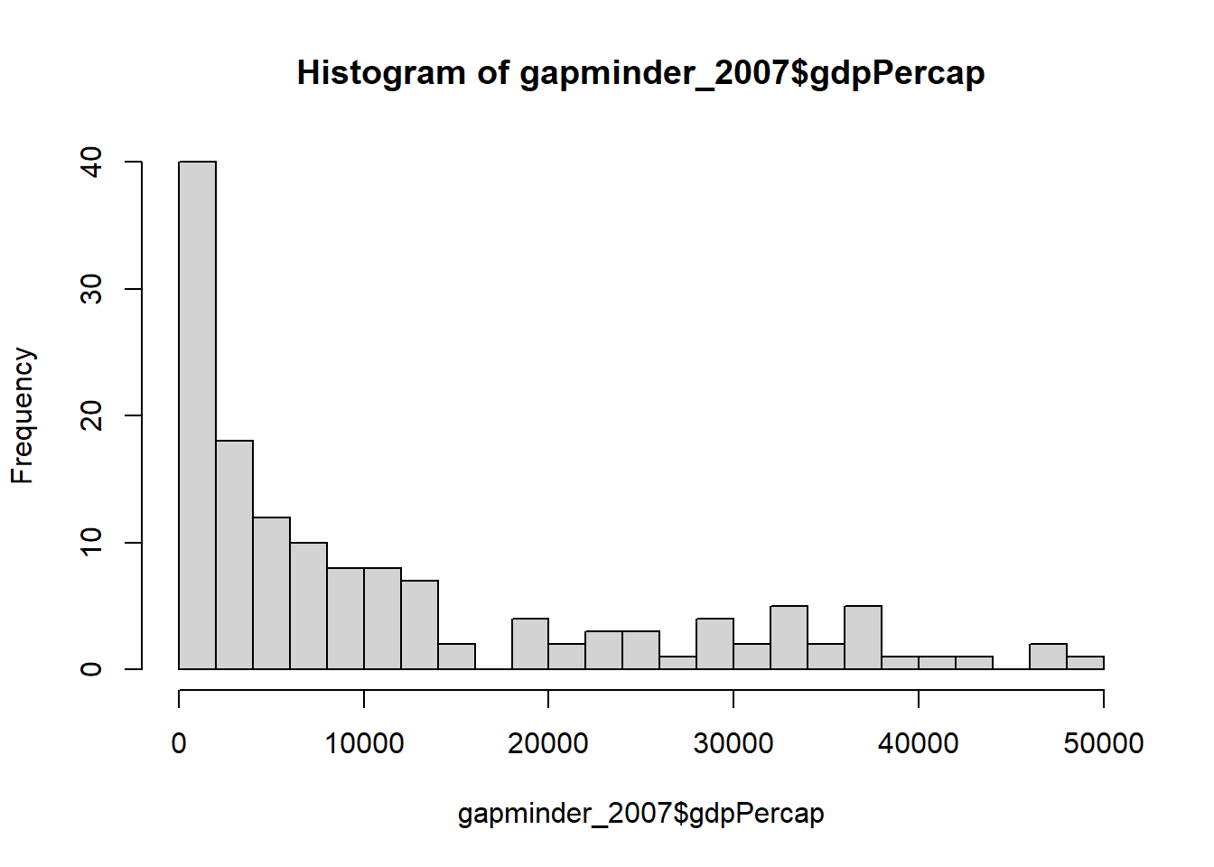
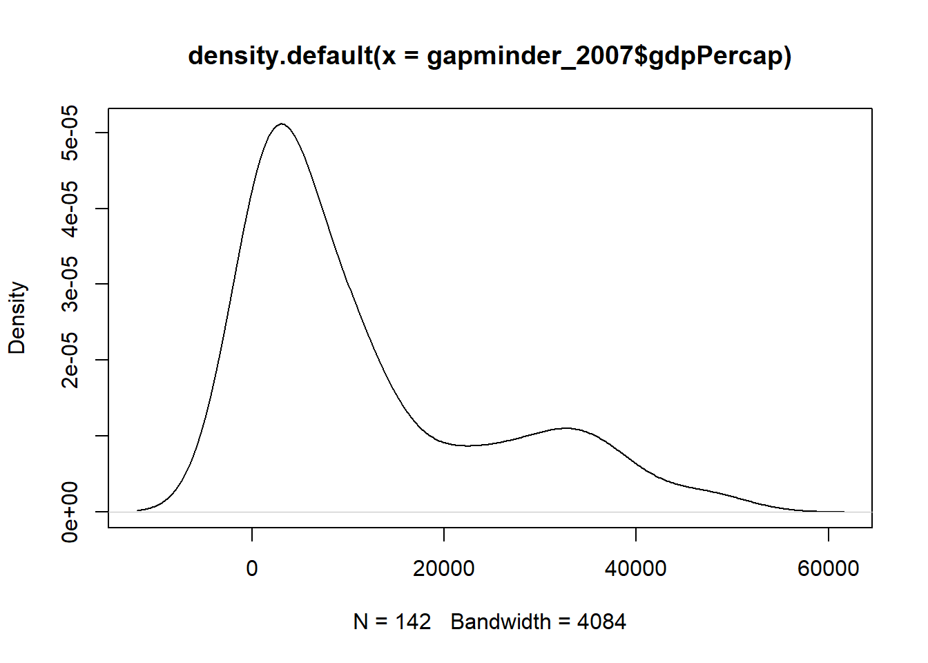
# boxplot of population
boxplot(gapminder_2007$gdpPercap)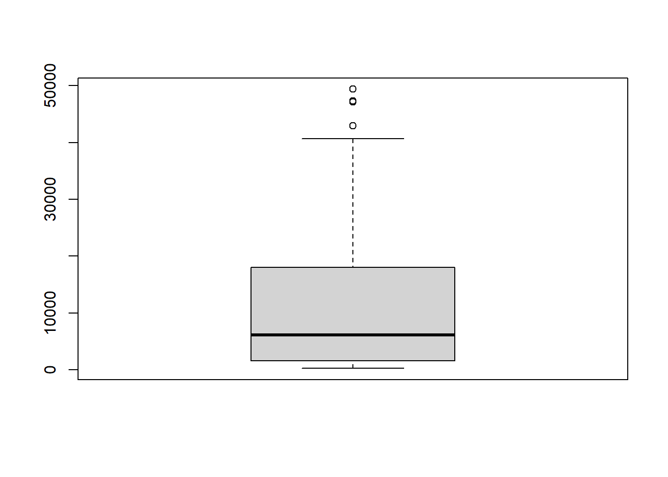
Of the above data visualizations, the boxplot is the most relevant as it shows both the spread of data and outliers. The boxplot reveals the following:
- minimum value,
- first quantile (Q1),
- median (second quantile),
- third quantile (Q3),
- maximum value excluding outliers and
- outliers.
The difference between Q3 and Q1 is known as the Interquartile Range (IQR).
The outliers within the box plot are calculated as any value that falls beyond 1.5 * IQR.
The function boxplot.stats() computes the data that is used to draw the box plot. Using this function, we can get our outliers.
boxplot.stats(gapminder_2007$gdpPercap)
#> $stats
#> [1]   277.5519  1598.4351  6124.3711 18008.9444 40675.9964
#>
#> $n
#> [1] 142
#>
#> $conf
#> [1] 3948.491 8300.251
#>
#> $out
#> [1] 47306.99 49357.19 47143.18 42951.65
The first element returned is the summary statistic as was calculated with summary().
boxplot.stats(gapminder_2007$gdpPercap)$stats
#> [1]   277.5519  1598.4351  6124.3711 18008.9444 40675.9964
summary(gapminder_2007$gdpPercap)
#>    Min. 1st Qu.  Median    Mean 3rd Qu.    Max.
#>   277.6  1624.8  6124.4 11680.1 18008.8 49357.2
The last element returned are the outliers.
boxplot.stats(gapminder_2007$gdpPercap)$out
#> [1] 47306.99 49357.19 47143.18 42951.65
Recall outliers are calculated as 1.5 * IQR, this can be changed using the argument coef. By default, it is set to 1.5 but can be changed as need be.
# changing coef
boxplot.stats(gapminder_2007$gdpPercap, coef = 0.8)$out
#>  [1] 34435.37 36126.49 33692.61 36319.24 35278.42 33207.08
#>  [7] 32170.37 39724.98 36180.79 40676.00 31656.07 47306.99
#> [13] 36797.93 49357.19 47143.18 33859.75 37506.42 33203.26
#> [19] 42951.65
boxplot.stats(gapminder_2007$gdpPercap, coef = 1)$out
#>  [1] 34435.37 36126.49 36319.24 35278.42 39724.98 36180.79
#>  [7] 40676.00 47306.99 36797.93 49357.19 47143.18 37506.42
#> [13] 42951.65
boxplot.stats(gapminder_2007$gdpPercap, coef = 1.2)$out
#> [1] 39724.98 40676.00 47306.99 49357.19 47143.18 42951.65

# selecting outliers
subset(gapminder_2007, gdpPercap >= min(boxplot.stats(gdpPercap)$out))
#> # A tibble: 4 x 5
#>   country       continent lifeExp       pop gdpPercap
#>   <fct>         <fct>       <dbl>     <int>     <dbl>
#> 1 Kuwait        Asia         77.6   2505559    47307.
#> 2 Norway        Europe       80.2   4627926    49357.
#> 3 Singapore     Asia         80.0   4553009    47143.
#> 4 United States Americas     78.2 301139947    42952.
5.13.4 Outliers by groups
# boxplot by continent
boxplot(gdpPercap ~ continent, gapminder_2007)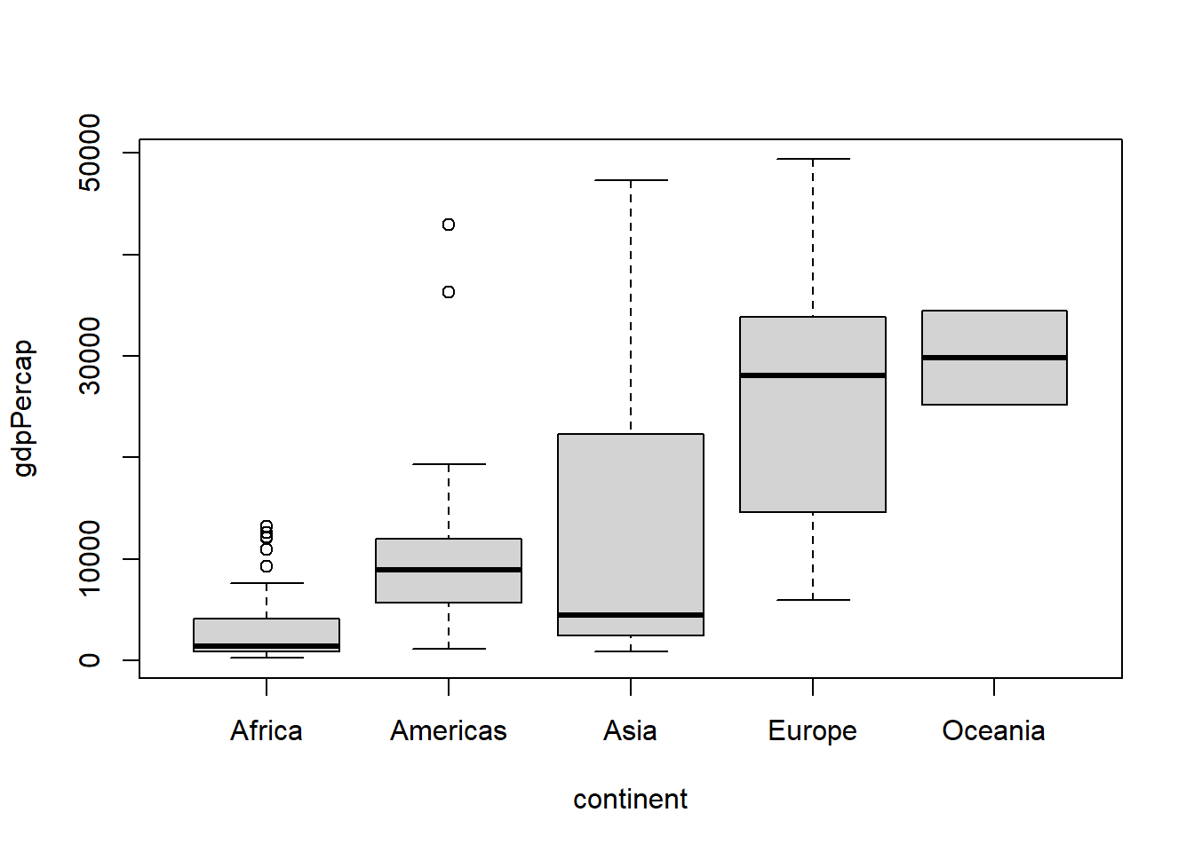
# splitting data frame
gap_split <- split(gapminder_2007, gapminder_2007$continent)

outliers_2007 <-
lapply(gap_split, function(x) {
    x <- boxplot.stats(x$gdpPercap)$out
    return(x)
})
outliers_2007
#> $Africa
#> [1] 12569.852 12154.090 13206.485 12057.499 10956.991
#> [6]  9269.658
#>
#> $Americas
#> [1] 36319.24 42951.65
#>
#> $Asia
#> numeric(0)
#>
#> $Europe
#> numeric(0)
#>
#> $Oceania
#> numeric(0)
5.14 String manipulation with stringr
5.14.1 Determine string length
The function str_length() returns the count of letters in a string.
library(stringr)
month.name
#>  [1] "January"   "February"  "March"     "April"
#>  [5] "May"       "June"      "July"      "August"
#>  [9] "September" "October"   "November"  "December"
str_length(month.name)
#>  [1] 7 8 5 5 3 4 4 6 9 7 8 8
5.14.2 Strings formatting (case conversion)
The functions str_to_upper(), str_to_lower(), str_to_title() and str_to_sentence() are used to convert to upper, lower, title and sentence cases respectively.
The function str_pad() is used to pad characters before and/or after a string.
The function str_trunc() is used to truncate a string.
# lowercase
str_to_lower('It is an everyday thing', locale = "en")
#> [1] "it is an everyday thing"

# uppercase
str_to_upper('It is an everyday thing', locale = "en")
#> [1] "IT IS AN EVERYDAY THING"

# title case
str_to_title('It is an everyday thing', locale = "en")
#> [1] "It Is An Everyday Thing"

# sentence case
str_to_sentence('iT is aN everyDay thIng', locale = "en")
#> [1] "It is an everyday thing"

# padding string
str_pad(c(12, 235, 'abd', 'ame'), width = 5, pad = '0')
#> [1] "00012" "00235" "00abd" "00ame"
str_pad(c(12, 235, 'abd', 'ame'), width = 5, pad = 'X', side = 'right')
#> [1] "12XXX" "235XX" "abdXX" "ameXX"
str_pad(c(12, 235, 'abd', 'ame'), width = 5, pad = '-', side = 'both')
#> [1] "-12--" "-235-" "-abd-" "-ame-"

# truncate a character string
str_trunc(state.name[1:8], width = 6)
#> [1] "Ala..." "Alaska" "Ari..." "Ark..." "Cal..." "Col..."
#> [7] "Con..." "Del..."
str_trunc(state.name[1:8], 6, side  = 'left')
#> [1] "...ama" "Alaska" "...ona" "...sas" "...nia" "...ado"
#> [7] "...cut" "...are"
str_trunc(state.name[1:8], 6, side  = 'right', ellipsis = '')
#> [1] "Alabam" "Alaska" "Arizon" "Arkans" "Califo" "Colora"
#> [7] "Connec" "Delawa"
5.14.3 Join and Split strings
5.14.3.1 joining strings with str_c()
The function str_c() joins two or more vectors element wise into a single character vector, optionally inserting separator (sep) between input vectors.
# combining elements into a character vector
str_c('a', 'b')
#> [1] "ab"
str_c(1, 2, 3, 4)
#> [1] "1234"

# using sep
str_c('a', 'b', sep = ' ')
#> [1] "a b"
str_c(1, 2, 3, 4, sep = ' ')
#> [1] "1 2 3 4"
str_c(1:10, sep = ' ')
#>  [1] "1"  "2"  "3"  "4"  "5"  "6"  "7"  "8"  "9"  "10"

# on a single vector
str_c(c('a', 'b'), sep = ' <> ')
#> [1] "a" "b"
str_c(c(1, 2), sep = ' <> ')
#> [1] "1" "2"

# two or more vectors
str_c(c('a', 'b'), c('c', 'd'), sep = ' <> ')
#> [1] "a <> c" "b <> d"
str_c(1:5, 10:20, sep = ' ')
#>  [1] "1 10" "2 11" "3 12" "4 13" "5 14" "1 15" "2 16" "3 17"
#>  [9] "4 18" "5 19" "1 20"
str_c(1:5, 10:20, c('a','b','c'), sep = ' ')
#>  [1] "1 10 a" "2 11 b" "3 12 c" "4 13 a" "5 14 b" "1 15 c"
#>  [7] "2 16 a" "3 17 b" "4 18 c" "5 19 a" "1 20 b"
# collapsing vectors
str_c(1:10, collapse = '~')
#> [1] "1~2~3~4~5~6~7~8~9~10"
str_c(c('a', 'b'), c('c', 'd'), collapse = ' <> ')
#> [1] "ac <> bd"
str_c(month.name[1:6], collapse = " - ")
#> [1] "January - February - March - April - May - June"

a <- month.name[1]
b <- month.name[2]
c <- month.name[3]

# combining character and variables
str_c(b,'comes after', a ,'but comes before', c, sep = " ")
#> [1] "February comes after January but comes before March"
str_c(b,'comes after', a ,'but comes before', c, sep = "/")
#> [1] "February/comes after/January/but comes before/March"
str_c('version 1.', 1:5, sep = '')
#> [1] "version 1.1" "version 1.2" "version 1.3" "version 1.4"
#> [5] "version 1.5"
5.14.4 Joining using str_glue()
The function str_glue() returns a character vector containing a formatted combination of text and variable values.
formatting with integers
x <- 2
str_glue('{x} * {x} = {x ** 2}')
#> 2 * 2 = 4

x <- c(1:4)
str_glue('{x} squared is equal to {x ** 2}')
#> 1 squared is equal to 1
#> 2 squared is equal to 4
#> 3 squared is equal to 9
#> 4 squared is equal to 16

num <- c(123, 1, 100, 200, 10200, 25000)
str_glue('my registration number is {str_pad(num, 5, pad = "0")}')
#> my registration number is 00123
#> my registration number is 00001
#> my registration number is 00100
#> my registration number is 00200
#> my registration number is 10200
#> my registration number is 25000
Formatting with strings
x <- 'my name is'
y <- 'james'
z <- 'london'
str_glue('{x} {y} and i live and work in {z}')
#> my name is james and i live and work in london


x <- 'my name is'
y <- 'james'
z <- 35
str_glue('{str_to_title(x)} {str_to_upper(y)} and i am {z} years')
#> My Name Is JAMES and i am 35 years

names <- c('paul', 'alphonse', 'michael', 'james', 'samson', 'terence', 'derin')
age <- c(30, 35, 32, 37, 29, 40, 30)
str_glue('i am {str_to_title(names)} and i am {age} years old')
#> i am Paul and i am 30 years old
#> i am Alphonse and i am 35 years old
#> i am Michael and i am 32 years old
#> i am James and i am 37 years old
#> i am Samson and i am 29 years old
#> i am Terence and i am 40 years old
#> i am Derin and i am 30 years old
Formatting with doubles or floating points
x <- 1000/6
x
#> [1] 166.6667
str_glue('1000 divided by 3 is {x}')
#> 1000 divided by 3 is 166.666666666667
str_glue('1000 divided by 3 is {round(x, 3)}')
#> 1000 divided by 3 is 166.667
str_glue('1000 divided by 3 is {round(x)}')
#> 1000 divided by 3 is 167
str_glue('1000 divided by 3 is {paste0("+", round(x))}')
#> 1000 divided by 3 is +167
str_glue('1000 divided by 3 is{paste0(" ", round(x))}')
#> 1000 divided by 3 is 167
5.14.5 Splitting strings using str_split() and str_split_fixed()
The function str_split() splits the elements of a character vector into substrings by a specific pattern.
The function str_split_fixed() splits up the elements of a character into a fixed number of pieces.
str(str_split(c('2020-01-01', '2019-03-31', '2018-06-30'), pattern = "-"))
#> List of 3
#>  $ : chr [1:3] "2020" "01" "01"
#>  $ : chr [1:3] "2019" "03" "31"
#>  $ : chr [1:3] "2018" "06" "30"
str(str_split(c('2020 01 01', '2019 03 31', '2018 06 30'), pattern = " "))
#> List of 3
#>  $ : chr [1:3] "2020" "01" "01"
#>  $ : chr [1:3] "2019" "03" "31"
#>  $ : chr [1:3] "2018" "06" "30"

# splitting into two substrings
str(str_split(c('2020-01-01', '2019-03-31', '2018-06-30'), pattern = "-", n = 2))
#> List of 3
#>  $ : chr [1:2] "2020" "01-01"
#>  $ : chr [1:2] "2019" "03-31"
#>  $ : chr [1:2] "2018" "06-30"
str(str_split(c('2020 01 01', '2019 03 31', '2018 06 30'), pattern = " ", n = 2))
#> List of 3
#>  $ : chr [1:2] "2020" "01 01"
#>  $ : chr [1:2] "2019" "03 31"
#>  $ : chr [1:2] "2018" "06 30"

# returning a matrix
str_split_fixed(c('2020-01-01', '2019-03-31', '2018-06-30'), '-', 2)
#>      [,1]   [,2]
#> [1,] "2020" "01-01"
#> [2,] "2019" "03-31"
#> [3,] "2018" "06-30"
str_split_fixed(c('2020-01-01', '2019-03-31', '2018-06-30'), '-', 3)
#>      [,1]   [,2] [,3]
#> [1,] "2020" "01" "01"
#> [2,] "2019" "03" "31"
#> [3,] "2018" "06" "30"
5.14.6 Extract and Replace part of a string
5.14.6.1 Extracting string values using str_sub()
The function str_sub() extracts a substring from a string by indexing. It uses start for the beginning position and stop for the ending position. It is like indexing but applied to a string.
var <- c('2020-01-01', '2019-03-31', '2018-06-30')
str_sub(var, start = 1, end = 4)
#> [1] "2020" "2019" "2018"
str_sub(var, 6, 7)
#> [1] "01" "03" "06"
str_sub(var, 9, 10)
#> [1] "01" "31" "30"

# using negative numbers
str_sub(var, -2, -1)
#> [1] "01" "31" "30"
str_sub(var, -5, -4)
#> [1] "01" "03" "06"
str_sub(var, -10, -7)
#> [1] "2020" "2019" "2018"
5.14.6.2 Replacing string values using str_sub()
The function str_sub() is also used to replace substring in a string by assigning a different string to the extracted substring.
5.14.7 Replacing string values using str_replace()
The function str_replace() replaces a substring at first occurrence.
var <- c('2020-01-01', '2019-03-31', '2018-06-30')
str_replace(var, "-", "")
#> [1] "202001-01" "201903-31" "201806-30"
str_replace(var, "-", "/")
#> [1] "2020/01-01" "2019/03-31" "2018/06-30"
5.14.8 Replacing string values using str_replace_all()
The function str_replace_all() replaces a substring throughout a string.
var <- c('2020-01-01', '2019-03-31', '2018-06-30')
str_replace_all(var, "-", " ")
#> [1] "2020 01 01" "2019 03 31" "2018 06 30"
str_replace_all(var, "-", "/")
#> [1] "2020/01/01" "2019/03/31" "2018/06/30"
5.14.8.1 Remove white spaces and clean string values
The function:
-
str_trim()removes white spaces. -
str_squish()removes repeated spaces. -
str_remove()removes the first repeated spaces. -
str_remove_all()removes all repeated spaces.
# both sides
str_trim(c(' 2020-01-01 ', ' 2019-03-31 ', ' 2018-06-30 '))
#> [1] "2020-01-01" "2019-03-31" "2018-06-30"

# left side
str_trim(c(' 2020-01-01 ', ' 2019-03-31 ', ' 2018-06-30 '), side = 'left')
#> [1] "2020-01-01 " "2019-03-31 " "2018-06-30 "

# right side
str_trim(c(' 2020-01-01 ', ' 2019-03-31 ', ' 2018-06-30 '), side = 'right')
#> [1] " 2020-01-01" " 2019-03-31" " 2018-06-30"

str_squish('removing   all    repeated   spaces in a string  ')
#> [1] "removing all repeated spaces in a string"

str_remove('removing   first  repeated   spaces in a string  ', '  ')
#> [1] "removing first  repeated   spaces in a string  "
str_remove_all('removing   all  repeated   spaces in a string  ', '  ')
#> [1] "removing allrepeated spaces in a string"
5.14.9 Sorting
The function:
-
str_order()sorts a character vector and returns sorted indices. -
str_sort()sorts a character vector and returns sorted values.
str_order(month.name)
#>  [1]  4  8 12  2  1  7  6  3  5 11 10  9
str_order(month.name, decreasing = T)
#>  [1]  9 10 11  5  3  6  7  1  2 12  8  4

str_sort(month.name)
#>  [1] "April"     "August"    "December"  "February"
#>  [5] "January"   "July"      "June"      "March"
#>  [9] "May"       "November"  "October"   "September"
str_sort(month.name, decreasing = T)
#>  [1] "September" "October"   "November"  "May"
#>  [5] "March"     "June"      "July"      "January"
#>  [9] "February"  "December"  "August"    "April"
5.14.10 Duplicating strings
The function str_dup() duplicates and concatenate strings within a character vector.
5.14.11 Pattern matching using regular expression
5.14.11.1 Regex functions
-
str_which(),str_detect()andstr_subset()` str_count()-
str_starts()andstr_ends() -
str_locate()andstr_locate_all() -
str_extract()andstr_extract_all() -
str_match()andstr_match_all() -
str_view()andstr_view_all() -
str_replace()andstr_replace_all()
5.14.11.1.1 The functions str_detect(), str_which() and str_subset()
The function:
-
str_detect()detects the presence or absence of a pattern in a string and is equivalent to grepl(pattern, x). -
str_which()detects the position of a matched pattern and is equivalent to grep(pattern, x). -
str_subset()keeps string matching a pattern and is equivalent to grep(pattern, x, value = TRUE).
str_detect(month.name, 'uary')
#>  [1]  TRUE  TRUE FALSE FALSE FALSE FALSE FALSE FALSE FALSE
#> [10] FALSE FALSE FALSE
month.name[str_detect(month.name, 'uary')]
#> [1] "January"  "February"
str_detect(month.name, 'uary', negate = T)
#>  [1] FALSE FALSE  TRUE  TRUE  TRUE  TRUE  TRUE  TRUE  TRUE
#> [10]  TRUE  TRUE  TRUE
month.name[str_detect(month.name, 'uary', negate = T)]
#>  [1] "March"     "April"     "May"       "June"
#>  [5] "July"      "August"    "September" "October"
#>  [9] "November"  "December"
str_which(month.name, 'uary')
#> [1] 1 2
month.name[str_which(month.name, 'uary')]
#> [1] "January"  "February"

str_which(month.name, 'uary', negate = T)
#>  [1]  3  4  5  6  7  8  9 10 11 12
month.name[str_which(month.name, 'uary', negate = T)]
#>  [1] "March"     "April"     "May"       "June"
#>  [5] "July"      "August"    "September" "October"
#>  [9] "November"  "December"

str_subset(month.name, pattern = 'ber')
#> [1] "September" "October"   "November"  "December"
str_subset(month.name, pattern = 'ber', negate = TRUE)
#> [1] "January"  "February" "March"    "April"    "May"
#> [6] "June"     "July"     "August"
5.14.11.1.2 The function str_count()
The function str_count() counts the number of matches in a string.
5.14.11.2 The functions str_starts() and str_ends()
The function:
-
str_starts()detects the presence of a pattern at the beginning of a string. -
str_ends()detects the presence of a pattern at the end of a string.
str_starts(month.name, 'J')
#>  [1]  TRUE FALSE FALSE FALSE FALSE  TRUE  TRUE FALSE FALSE
#> [10] FALSE FALSE FALSE
month.name[str_starts(month.name, 'J')]
#> [1] "January" "June"    "July"
str_ends(month.name, 'ber')
#>  [1] FALSE FALSE FALSE FALSE FALSE FALSE FALSE FALSE  TRUE
#> [10]  TRUE  TRUE  TRUE
month.name[str_ends(month.name, 'ber')]
#> [1] "September" "October"   "November"  "December"
5.14.11.2.1 The functions str_locate() and str_locate_all()
The function:
-
str_locate()locates the position of the first pattern match in a string. -
str_locate_all()locates the position of all pattern matches in a string.
str_locate(month.name, 'ber')
#>       start end
#>  [1,]    NA  NA
#>  [2,]    NA  NA
#>  [3,]    NA  NA
#>  [4,]    NA  NA
#>  [5,]    NA  NA
#>  [6,]    NA  NA
#>  [7,]    NA  NA
#>  [8,]    NA  NA
#>  [9,]     7   9
#> [10,]     5   7
#> [11,]     6   8
#> [12,]     6   8
5.14.11.2.2 The functions str_extract() and str_extract_all()
The function:
-
str_extract()extracts the first matching pattern from a string. -
str_extract_all()extracts all matching patterns from a string.
str_extract(string = month.name, pattern = 'ber')
#>  [1] NA    NA    NA    NA    NA    NA    NA    NA    "ber"
#> [10] "ber" "ber" "ber"
5.14.11.2.3 The functions str_view() and str_view_all()
The functions str_view() and str_view_all() Views HTML rendering of regular expression match, with the first matching the first occurrence and the later all occurrences.
str_view(month.name, 'uary')5.14.11.3 Regex Operations
matching spaces
var <- c('2020 01 01', '2019 03 31', '2018 06 30')
str_replace_all(var, '[[:space:]]', '-')
#> [1] "2020-01-01" "2019-03-31" "2018-06-30"
str_replace_all(var, '\\s', '-')
#> [1] "2020-01-01" "2019-03-31" "2018-06-30"
str(str_split(var, '\\s'))
#> List of 3
#>  $ : chr [1:3] "2020" "01" "01"
#>  $ : chr [1:3] "2019" "03" "31"
#>  $ : chr [1:3] "2018" "06" "30"
str_replace_all(var, '\\S', '-')
#> [1] "---- -- --" "---- -- --" "---- -- --"
matching alphabetic characters
var <- 'a1b2c3d4e5f'
str_replace_all(var, '[[:alpha:]]', '')
#> [1] "12345"
# lowercase letters
str_replace_all(month.name, '[[:lower:]]', '')
#>  [1] "J" "F" "M" "A" "M" "J" "J" "A" "S" "O" "N" "D"
matching numerical digits
var <- 'a1b2c3d4e5f'
str_replace_all(var, '[[:digit:]]', '')
#> [1] "abcdef"
str_replace_all(var, '\\d', '')
#> [1] "abcdef"
matching letters and numbers (alphanumeric characters)
var <- 'a1@; 2#4c $8`*%f^!1~0&^h*()j'
str_replace_all(var, '[[:alnum:]]', '')
#> [1] "@; # $`*%^!~&^*()"

str_replace_all(var, '[[:xdigit:]]', '')
#> [1] "@; # $`*%^!~&^h*()j"

str_replace_all(var, '\\w', '')
#> [1] "@; # $`*%^!~&^*()"
matching punctuation
var <- 'a1@; 2#4c $8`*%f^!1~0&^h*()j'
str_replace_all(var, '[[:punct:]]', '')
#> [1] "a1 24c $8`f^1~0^hj"

str_replace_all(var, '\\W', '')
#> [1] "a124c8f10hj"
matching letters, numbers, and punctuation
var <- 'a1@; 2#4c $8`*%f^!1~0&^h*()j'
str_replace_all(var, '[[:graph:]]', ' ')
#> [1] "                            "

str_replace_all(var, '.', ' ')
#> [1] "                            "
matching whitespace
str_replace_all(c(' 2020-01-01 ', ' 2019-03-31 ', ' 2018-06-30 '), '\\s', '')
#> [1] "2020-01-01" "2019-03-31" "2018-06-30"
matching newline and tap
cat('good morning \n i am fru kinglsy \n i will be your instructor')
#> good morning
#>  i am fru kinglsy
#>  i will be your instructor

# replacing new line
str_replace_all('good morning \n i am fru kinglsy \n i will be your instructor', '\\n', '\t')
#> [1] "good morning \t i am fru kinglsy \t i will be your instructor"
cat(str_replace_all('good morning \n i am fru kinglsy \n i will be your instructor', '\\n', '\t'))
#> good morning      i am fru kinglsy    i will be your instructor

# replacing tab
str_replace_all('good morning \t i am fru kinglsy \t i will be your instructor', '\\t', '\n')
#> [1] "good morning \n i am fru kinglsy \n i will be your instructor"
cat(str_replace_all('good morning \t i am fru kinglsy \t i will be your instructor', '\\t', '\n'))
#> good morning
#>  i am fru kinglsy
#>  i will be your instructor
matching metacharacters
sales <- c('$25000', '$20000', '$22500', '$24000', '$30000', '$35000')
str_replace(sales, '\\$', '')
#> [1] "25000" "20000" "22500" "24000" "30000" "35000"

sales <- c('+25000', '+20000', '+22500', '+24000', '+30000', '+35000')
str_replace(sales, '\\+', '')
#> [1] "25000" "20000" "22500" "24000" "30000" "35000"

dates <- c('01.01.2012', '01.02.2012', '01.03.2012', '01.04.2012', '01.05.2012', '01.06.2012')
str_replace_all(dates, '\\.', '-')
#> [1] "01-01-2012" "01-02-2012" "01-03-2012" "01-04-2012"
#> [5] "01-05-2012" "01-06-2012"

dates <- c('01*01*2012', '01*02*2012', '01*03*2012', '01*04*2012', '01*05*2012', '01*06*2012')
str_replace_all(dates, '\\*', '-')
#> [1] "01-01-2012" "01-02-2012" "01-03-2012" "01-04-2012"
#> [5] "01-05-2012" "01-06-2012"

dates <- c('01^01^2012', '01^02^2012', '01^03^2012', '01^04^2012', '01^05^2012', '01^06^2012')
str_replace_all(dates, '\\^', '-')
#> [1] "01-01-2012" "01-02-2012" "01-03-2012" "01-04-2012"
#> [5] "01-05-2012" "01-06-2012"

dates <- c('01|01|2012', '01|02|2012', '01|03|2012', '01|04|2012', '01|05|2012', '01|06|2012')
str_replace_all(dates, '\\|', '-')
#> [1] "01-01-2012" "01-02-2012" "01-03-2012" "01-04-2012"
#> [5] "01-05-2012" "01-06-2012"

dates <- c('01\\01\\2012', '01\\02\\2012', '01\\03\\2012', '01\\04\\2012', '01\\05\\2012', '01\\06\\2012')
str_replace_all(dates, '\\\\', '-')
#> [1] "01-01-2012" "01-02-2012" "01-03-2012" "01-04-2012"
#> [5] "01-05-2012" "01-06-2012"

dates <- c('01\\.01\\.2012', '01\\.02\\.2012', '01\\.03\\.2012', '01\\.04\\.2012', '01\\.05\\.2012', '01\\.06\\.2012')
str_replace_all(dates, '\\\\\\.', '-')
#> [1] "01-01-2012" "01-02-2012" "01-03-2012" "01-04-2012"
#> [5] "01-05-2012" "01-06-2012"
alternates and ranges
# either or
str_view_all(month.name, 'uary|ember|ober', '*')groups
str_subset(pattern = '(s{2})e', state.name)
#> [1] "Tennessee"
anchors
# start of a string
str_replace_all(month.name, '^J', 'j')
#>  [1] "january"   "February"  "March"     "April"
#>  [5] "May"       "june"      "july"      "August"
#>  [9] "September" "October"   "November"  "December"

# end of a string
str_replace_all(month.name, 'ber$', 'ba')
#>  [1] "January"  "February" "March"    "April"    "May"
#>  [6] "June"     "July"     "August"   "Septemba" "Octoba"
#> [11] "Novemba"  "Decemba"
quantifiers
# match 's' zero or one time
str_subset(month.name, 's?')
#>  [1] "January"   "February"  "March"     "April"
#>  [5] "May"       "June"      "July"      "August"
#>  [9] "September" "October"   "November"  "December"
# match 'J' one or more times
str_subset(month.name, 'J+')
#> [1] "January" "June"    "July"
# match 'e' one or more times
str_subset(state.name, 'e+')
#>  [1] "Connecticut"   "Delaware"      "Georgia"
#>  [4] "Kentucky"      "Maine"         "Massachusetts"
#>  [7] "Minnesota"     "Nebraska"      "Nevada"
#> [10] "New Hampshire" "New Jersey"    "New Mexico"
#> [13] "New York"      "Oregon"        "Pennsylvania"
#> [16] "Rhode Island"  "Tennessee"     "Texas"
#> [19] "Vermont"       "West Virginia"
# matched 'y', zero or more times
str_subset(month.name, 'y*')
#>  [1] "January"   "February"  "March"     "April"
#>  [5] "May"       "June"      "July"      "August"
#>  [9] "September" "October"   "November"  "December"
# matched 'a', zero or more times
str_subset(month.name, 'a*')
#>  [1] "January"   "February"  "March"     "April"
#>  [5] "May"       "June"      "July"      "August"
#>  [9] "September" "October"   "November"  "December"
# match 'a' zero or more times and 'y'
str_subset(month.name, 'a*y')
#> [1] "January"  "February" "May"      "July"
# match 'y' zero or more times and 'a'
str_subset(month.name, 'y*a')
#> [1] "January"  "February" "March"    "May"
# match 's', exactly 2 times
str_subset(state.name, "s{2}")
#> [1] "Massachusetts" "Mississippi"   "Missouri"
#> [4] "Tennessee"
# match 's', exactly 1 or more times
str_subset(state.name, "s{1,}")
#>  [1] "Alaska"        "Arkansas"      "Illinois"
#>  [4] "Kansas"        "Louisiana"     "Massachusetts"
#>  [7] "Minnesota"     "Mississippi"   "Missouri"
#> [10] "Nebraska"      "New Hampshire" "New Jersey"
#> [13] "Pennsylvania"  "Rhode Island"  "Tennessee"
#> [16] "Texas"         "Washington"    "West Virginia"
#> [19] "Wisconsin"
# match 's', exactly 1 or 2 times
str_subset(state.name, "s{1,2}")
#>  [1] "Alaska"        "Arkansas"      "Illinois"
#>  [4] "Kansas"        "Louisiana"     "Massachusetts"
#>  [7] "Minnesota"     "Mississippi"   "Missouri"
#> [10] "Nebraska"      "New Hampshire" "New Jersey"
#> [13] "Pennsylvania"  "Rhode Island"  "Tennessee"
#> [16] "Texas"         "Washington"    "West Virginia"
#> [19] "Wisconsin"