7 Bioconductor
7.1 Introduction
The Bioconductor project is an open source repository for R packages, datasets and workflows that are specific for analyzing biological data. The Bioconductor project is a useful extension on CRAN, the R Archive, because it provides us with the software tools to explore, understand, and solve simple and complex molecular biology questions. Hence, Bioconductor’s tagline is “open source software for bioinformatics.”
Bioconductor site: https://www.bioconductor.org/
7.2 How to install Bioconductor packages?
The Bioconductor package collection forms its own repository and has a release schedule different from the R Archive. Because Bioconductor has it’s own base functions and updates, packages are installed differently. To install Bioconductor packages you need some lines of code, as shown below.
if (!requireNamespace("BiocManager", quietly = TRUE))
    install.packages("BiocManager")
BiocManager::install()                  # install core packages
BiocManager::install("GenomicFeatures") # install GenomicFeatures package
First, use the function install.packages("BiocManager"). This function will install the BiocInstaller package. Then, use the function BiocManager::install() with the name of the package you want to install. Once you use BiocManager::install(), you will be informed if any new versions of Bioconductor are available, and will also see a prompt to update your R version if needed. Updating packages, regularly, is important to get the new features. In case there are upgrades on packages or dependencies, you will be asked to update all, some, or none of the packages.
7.2.1 Bioconductor version and package version
Because Bioconductor is in constant development, you can check the version of Bioconductor using the syntax BiocManager::version(). To load a package use the function library() like with CRAN packages. It’s important for reproducibility to always check the versions of your packages. You can use the function sessionInfo() which gives you a list of all the loaded packages and their versions, or you can inquire the version of each package using packageVersion() and the packageName. Finally, if you are interested to know if you have out-of-date packages, use the function BiocManager::valid().
version                  # detailed information about the version of R running
sessionInfo()            # version information about R, the OS and attached or loaded packages
BiocManager::version()   # version of Bioconductor currently in use
BiocManager::valid()     # Validate installed package versions against correct versions
packageVersion("GenomicFeatures")  # package version

# to install some new packages
.libPaths()
BiocManager::install(c(
    "backports", "Cairo", "loo", "openssl", "Rcpp", "svglite", "vdiffr"
  ), update = TRUE, ask = FALSE)
BSgenome is a Bioconductor data package that contains representations of several genomes. This package has already been installed for you, as installing the dependencies usually takes some time, using the following code:
7.3 OO systems
R is a functional programming language, which means we are working with a series of functions. We achieve our goal by sequencing or nested function calls. The use of Tidyverse R and the pipe operator greatly facilitates the interpretation and modification of multiple nested functions.
However, R also has object-oriented capabilities, so our capabilities expand greatly when using R.
In R you can use several object-oriented systems in parallel (more details https://adv-r.hadley.nz/oo.html):
- S3 - the simplest OO system, tied to basic data types
- S4 - Bioconductor is being developed in this (details: S4 System Development in Bioconductor and S4 classes and methods
- RC - Reference classes, the latest OO system in R (from version 2.12 R)
We review two object-oriented systems, systems S3 and S4. Most of the R packets use the S3 system, the Bioconductor handles the S4.
7.3.1 S3
Advantages of S3:
- simple but powerful
- flexible and interactive
- uses a generic function
- functionality depends on the first argument.
A good example of S3 is the plot () function, which can draw more than 30 different figures, depending on the input.
methods(plot) # List Methods for S3 Generic Functions or Classes of plot()
#>  [1] plot,ANY,ANY-method
#>  [2] plot,profile.mle,missing-method
#>  [3] plot.acf*
#>  [4] plot.data.frame*
#>  [5] plot.decomposed.ts*
#>  [6] plot.default
#>  [7] plot.dendrogram*
#>  [8] plot.density*
#>  [9] plot.ecdf
#> [10] plot.factor*
#> [11] plot.formula*
#> [12] plot.function
#> [13] plot.hclust*
#> [14] plot.histogram*
#> [15] plot.HoltWinters*
#> [16] plot.isoreg*
#> [17] plot.lm*
#> [18] plot.medpolish*
#> [19] plot.mlm*
#> [20] plot.ppr*
#> [21] plot.prcomp*
#> [22] plot.princomp*
#> [23] plot.profile.nls*
#> [24] plot.R6*
#> [25] plot.raster*
#> [26] plot.shingle*
#> [27] plot.spec*
#> [28] plot.stepfun
#> [29] plot.stl*
#> [30] plot.table*
#> [31] plot.trellis*
#> [32] plot.ts
#> [33] plot.tskernel*
#> [34] plot.TukeyHSD*
#> see '?methods' for accessing help and source code
x <- rbinom(n = 10, size = 4, prob = 0.5)
plot(x)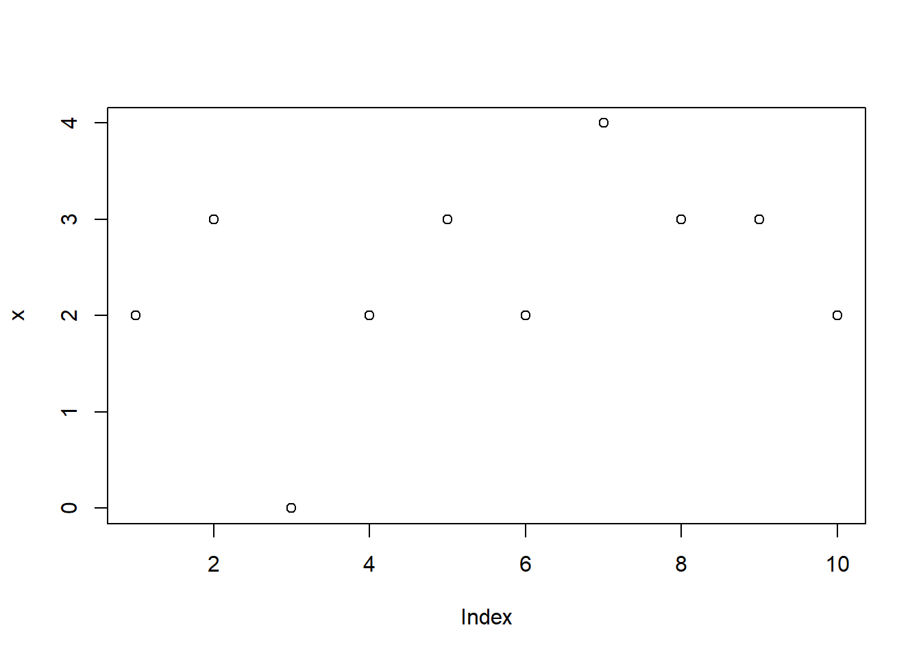

However, the S3 is not strong in type evaluation and selection. For example, if you give a function the wrong type, it will try all of them before printing the error. Naming difficulties (dot or not dot) and inheritance work, but it depends on the input.
7.3.1.1 Bases
S3 is the most widely used object-oriented system in CRAN packages. The base and stats packages only use this system.
Each S3 object has a class attribute, but of course it can have other attributes to store different information.
f <- factor(c("a", "b", "c"))
typeof(f)     # The Type of an Object
#> [1] "integer"
attributes(f) # Object Attribute Lists
#> $levels
#> [1] "a" "b" "c"
#>
#> $class
#> [1] "factor"
unclass(f)    # returns f with its class attribute removed
#> [1] 1 2 3
#> attr(,"levels")
#> [1] "a" "b" "c"
sloop::otype(f) # Determine the type of an object
#> [1] "S3"
There are generic functions in R that define an interface that uses a different implementation depending on the argument received. Most R functions are generic, such as print () and the plot () seen earlier.
print(f)
#> [1] a b c
#> Levels: a b c
print(unclass(f))
#> [1] 1 2 3
#> attr(,"levels")
#> [1] "a" "b" "c"
We can know whether any function is generic or not.
sloop::ftype(str)    # Determine function type.
#> [1] "S3"      "generic"
sloop::ftype(print)
#> [1] "S3"      "generic"
sloop::ftype(unclass)
#> [1] "primitive"
sloop::ftype(mean)
#> [1] "S4"      "generic"
The class of the S3 object is printed by class (), but inherits () provides a logical value if the object is an instance of that class.
The job of an S3 generic is to perform method dispatch, i.e. find the specific implementation for a class. Method dispatch is performed by UseMethod(), which every generic calls. How does UseMethod() work? It basically creates a vector of method names, paste0("generic", ".", c(class(x), "default")), and then looks for each potential method in turn. We can see this in action with sloop::s3_dispatch(). You give it a call to an S3 generic, and it lists all the possible methods.
sloop::s3_dispatch(print(f))
#> => print.factor
#>  * print.default
7.3.1.2 Classes
In the S3 system, there is no formal definition of objects. If you want to create your own class, you need to specify the class attribute. You can also create an object of a class with the structure () function or later with the class () function.
x <- structure(1:10, class="my_class")
sloop::otype(x)
#> [1] "S3"

x <- 1:10
class(x) <- "my_class"
x
#>  [1]  1  2  3  4  5  6  7  8  9 10
#> attr(,"class")
#> [1] "my_class"
sloop::otype(x)
#> [1] "S3"
The class of the S3 object is printed by class (), but inherits () provides a logical value if the object is an instance of that class.
It is very easy to ruin an existing object by modifying the class.
7.3.2 S4
The S4 system motivation is to implement an object-oriented style of programming. The base concept is to define the data first and then work on it. Once an object is defined, it is generalized to a class by defining the kind of data it contains and any actions or functions to manipulate it. As you will see in more detail in the coming chapters, biological representations are complex and very often interconnected. Bioconductor then, recommends re-using methods and classes before implementing new representations. S4 classes have a formal definition, hence are a lot better to check input types, because of their definition and inheritance. You can create a new object from a class like in the example. We created a new genome description. This object will contain slots to describe it. S4 requires a bit more work to implement, but it serves to extend the code so that others can reuse the framework.
Benefits of S4
- formal definition of classes
- Bioconductor reusability
- has validation of types
- naming conventions.
Use the new () function to create a new object. The object will contain slots to describe the data. The S4 system is a bit more complex than the S3.
It is easy to decide whether an object is an object defined in S4 or not. This can also be said by the isS4 () or str () functions. In the first case TRUE is displayed and in the second caseFormal class.
mydescr <- new("GenomeDescription") # create a new object from a class
isS4(mydescr)
#> [1] TRUE
isS4(mean(1:10))
#> [1] FALSE
str(mydescr)
#> Formal class 'GenomeDescription' [package "GenomeInfoDb"] with 7 slots
#>   ..@ organism        : chr(0)
#>   ..@ common_name     : chr(0)
#>   ..@ provider        : chr(0)
#>   ..@ provider_version: chr(0)
#>   ..@ release_date    : chr(0)
#>   ..@ release_name    : chr(0)
#>   ..@ seqinfo         :Formal class 'Seqinfo' [package "GenomeInfoDb"] with 4 slots
#>   .. .. ..@ seqnames   : chr(0)
#>   .. .. ..@ seqlengths : int(0)
#>   .. .. ..@ is_circular: logi(0)
#>   .. .. ..@ genome     : chr(0)
We can use the function sloop::otype().
sloop::otype(mydescr)
#> [1] "S4"
attributes(mydescr)
#> $organism
#> character(0)
#>
#> $common_name
#> character(0)
#>
#> $provider
#> character(0)
#>
#> $provider_version
#> character(0)
#>
#> $release_date
#> character(0)
#>
#> $release_name
#> character(0)
#>
#> $seqinfo
#> Seqinfo object with no sequences:
#>
#> $class
#> [1] "GenomeDescription"
#> attr(,"package")
#> [1] "GenomeInfoDb"
7.3.2.1 S4 class definition
An S4 class describes a representation of an object with a name and slots (also called methods or fields). A class optionally describes its inheritance. A class allows us to define all the characteristics concerning an object and it gives us code reusability. For example, we create a class using setClass(). Its name is MyEpicProject with three slots: ini, end and milestone. This class inherits from the class MyProject. This means we can reuse slots from it.
MyEpicProject <- setClass(
  "MyEpicProject",        # define class name with UpperCamelCase
  slots = c(ini = "Date", # define slots, helpful for validation
            end = "Date",
            milestone = "character"),
  contains = "MyProject" # define inheritance
)
S4 class definition
A class describes a representation:
- name
- slots (methids/fields)
- contains (inheritance definition)
7.3.2.2 S4 accessors
Basic information of an S4 object is accessed through accessor-functions, also called methods. As we have seen, a class definition includes slots for describing an object. The function .S4methods() used with main classes gives you a summary of its accessors. For other subclasses use the showMethods() function, but this gives you a breakdown, which might be a bit too long to look at. If you want an object summary, use the accessor function show(). You will use some of these accessors in the coming exercises.
We will use the class BSgenome, which is already loaded for you. Let’s check the formal definition of this class by using the function showClass("className"). Check the BSgenome class results and find its parent classes (Extends) and the classes that inherit from it (Subclasses).
library(BSgenome) # load the package
.S4methods(class = "BSgenome") # accessors from the main class
#>  [1] $               [[              as.list
#>  [4] coerce          commonName      countPWM
#>  [7] export          extractAt       getSeq
#> [10] injectSNPs      length          masknames
#> [13] matchPWM        mseqnames       names
#> [16] organism        provider        providerVersion
#> [19] releaseDate     releaseName     seqinfo
#> [22] seqinfo<-       seqnames        seqnames<-
#> [25] show            snpcount        snplocs
#> [28] SNPlocs_pkgname sourceUrl       vcountPattern
#> [31] Views           vmatchPattern   vcountPDict
#> [34] vmatchPDict     bsgenomeName    metadata
#> [37] metadata<-
#> see '?methods' for accessing help and source code
#showMethods(classes = "BSgenome") # too long output
showClass("BSgenome") # parents and children
#> Class "BSgenome" [package "BSgenome"]
#>
#> Slots:
#>
#> Name:               pkgname     single_sequences
#> Class:            character OnDiskNamedSequences
#>
#> Name:    multiple_sequences              seqinfo
#> Class:        RdaCollection              Seqinfo
#>
#> Name:         user_seqnames   injectSNPs_handler
#> Class:            character    InjectSNPsHandler
#>
#> Name:           .seqs_cache         .link_counts
#> Class:          environment          environment
#>
#> Name:              metadata
#> Class:                 list
#>
#> Extends: "Annotated"
#>
#> Known Subclasses: "MaskedBSgenome"

# new object and object summary
setClass("track", slots = c(x="numeric", y="numeric"))
t1 <- new("track", x=1:20, y=(1:20)^2)
show(t1)
#> An object of class "track"
#> Slot "x":
#>  [1]  1  2  3  4  5  6  7  8  9 10 11 12 13 14 15 16 17 18
#> [19] 19 20
#>
#> Slot "y":
#>  [1]   1   4   9  16  25  36  49  64  81 100 121 144 169 196
#> [15] 225 256 289 324 361 400
The BSgenome is a powerful class and inherits from Annotated, which you will see later on, and has MaskedBSgenome as subclass.
7.4 Introducing genomic datasets
All organisms have a genome which makes up what they are, and it dictates responses to external influences. A genome is the complete genetic material of an organism stored mostly in the chromosomes, it’s known as the blueprint of the living. A genome is made of long sequences of DNA, based on a four-letter-alphabet, T, A, G and C.
We are interested in locating and describing specific locations in a genome because this allows us to learn about diversity, evolution, hereditary changes, and more. To understand this better we subdivide a genome. The written information in a genome uses the DNA alphabet. Think of a genome as a set of books and each book is a chromosome. Chromosome numbers on each genome are highly variable. Usually, chromosomes come in pairs, but multiple sets are very common too. Each chromosome has ordered genetic sequences, think of chapters in a book. To find specific genetic instructions we look at genes. These are like the pages in a book, containing a recipe to make proteins. Some genes will produce proteins but some won’t. These are called coding and non-coding genes. Coding genes are expressed through proteins responsible for specific functions. Proteins come up following a two-step process, DNA-to-RNA, a step known as transcription, while the RNA-to-protein is a step called translation.
As an example, we are going to study the Yeast genome, a single cell microorganism. The fungus that people love. Yeast is used for fermentation and production of beer, bread, kefir, kombucha and other foods, as well as used for bioremediation. Its scientific name is Saccharomyces cerevisiae or s. cerevisiae. Yeast is a very well studied organism, due to its fast development, many experiments use it as model.
7.4.1 Yeast genome
The yeast genome is a dataset available from UCSC. We have picked this genome because it has a small size. The BSgenome package provides us with many genome datasets. To get a list of the BSgenome available datasets, use the function available.genomes(). Then, using common accessors functions, you can learn about the genome, for example, the number of chromosomes using length(), the names of the chromosomes using names(), and the length of each chromosome by DNA base pairs, using seqlengths().
# BiocManager::install("BSgenome.Scerevisiae.UCSC.sacCer3")
# Load the yeast genome
library(BSgenome.Scerevisiae.UCSC.sacCer3)

# Assign data to the yeastGenome object
yeastGenome <- BSgenome.Scerevisiae.UCSC.sacCer3

# interested in other genomes
available.genomes()
#>   [1] "BSgenome.Alyrata.JGI.v1"
#>   [2] "BSgenome.Amellifera.BeeBase.assembly4"
#>   [3] "BSgenome.Amellifera.NCBI.AmelHAv3.1"
#>   [4] "BSgenome.Amellifera.UCSC.apiMel2"
#>   [5] "BSgenome.Amellifera.UCSC.apiMel2.masked"
#>   [6] "BSgenome.Aofficinalis.NCBI.V1"
#>   [7] "BSgenome.Athaliana.TAIR.04232008"
#>   [8] "BSgenome.Athaliana.TAIR.TAIR9"
#>   [9] "BSgenome.Btaurus.UCSC.bosTau3"
#>  [10] "BSgenome.Btaurus.UCSC.bosTau3.masked"
#>  [11] "BSgenome.Btaurus.UCSC.bosTau4"
#>  [12] "BSgenome.Btaurus.UCSC.bosTau4.masked"
#>  [13] "BSgenome.Btaurus.UCSC.bosTau6"
#>  [14] "BSgenome.Btaurus.UCSC.bosTau6.masked"
#>  [15] "BSgenome.Btaurus.UCSC.bosTau8"
#>  [16] "BSgenome.Btaurus.UCSC.bosTau9"
#>  [17] "BSgenome.Carietinum.NCBI.v1"
#>  [18] "BSgenome.Celegans.UCSC.ce10"
#>  [19] "BSgenome.Celegans.UCSC.ce11"
#>  [20] "BSgenome.Celegans.UCSC.ce2"
#>  [21] "BSgenome.Celegans.UCSC.ce6"
#>  [22] "BSgenome.Cfamiliaris.UCSC.canFam2"
#>  [23] "BSgenome.Cfamiliaris.UCSC.canFam2.masked"
#>  [24] "BSgenome.Cfamiliaris.UCSC.canFam3"
#>  [25] "BSgenome.Cfamiliaris.UCSC.canFam3.masked"
#>  [26] "BSgenome.Cjacchus.UCSC.calJac3"
#>  [27] "BSgenome.Creinhardtii.JGI.v5.6"
#>  [28] "BSgenome.Dmelanogaster.UCSC.dm2"
#>  [29] "BSgenome.Dmelanogaster.UCSC.dm2.masked"
#>  [30] "BSgenome.Dmelanogaster.UCSC.dm3"
#>  [31] "BSgenome.Dmelanogaster.UCSC.dm3.masked"
#>  [32] "BSgenome.Dmelanogaster.UCSC.dm6"
#>  [33] "BSgenome.Drerio.UCSC.danRer10"
#>  [34] "BSgenome.Drerio.UCSC.danRer11"
#>  [35] "BSgenome.Drerio.UCSC.danRer5"
#>  [36] "BSgenome.Drerio.UCSC.danRer5.masked"
#>  [37] "BSgenome.Drerio.UCSC.danRer6"
#>  [38] "BSgenome.Drerio.UCSC.danRer6.masked"
#>  [39] "BSgenome.Drerio.UCSC.danRer7"
#>  [40] "BSgenome.Drerio.UCSC.danRer7.masked"
#>  [41] "BSgenome.Dvirilis.Ensembl.dvircaf1"
#>  [42] "BSgenome.Ecoli.NCBI.20080805"
#>  [43] "BSgenome.Gaculeatus.UCSC.gasAcu1"
#>  [44] "BSgenome.Gaculeatus.UCSC.gasAcu1.masked"
#>  [45] "BSgenome.Ggallus.UCSC.galGal3"
#>  [46] "BSgenome.Ggallus.UCSC.galGal3.masked"
#>  [47] "BSgenome.Ggallus.UCSC.galGal4"
#>  [48] "BSgenome.Ggallus.UCSC.galGal4.masked"
#>  [49] "BSgenome.Ggallus.UCSC.galGal5"
#>  [50] "BSgenome.Ggallus.UCSC.galGal6"
#>  [51] "BSgenome.Hsapiens.1000genomes.hs37d5"
#>  [52] "BSgenome.Hsapiens.NCBI.GRCh38"
#>  [53] "BSgenome.Hsapiens.UCSC.hg17"
#>  [54] "BSgenome.Hsapiens.UCSC.hg17.masked"
#>  [55] "BSgenome.Hsapiens.UCSC.hg18"
#>  [56] "BSgenome.Hsapiens.UCSC.hg18.masked"
#>  [57] "BSgenome.Hsapiens.UCSC.hg19"
#>  [58] "BSgenome.Hsapiens.UCSC.hg19.masked"
#>  [59] "BSgenome.Hsapiens.UCSC.hg38"
#>  [60] "BSgenome.Hsapiens.UCSC.hg38.dbSNP151.major"
#>  [61] "BSgenome.Hsapiens.UCSC.hg38.dbSNP151.minor"
#>  [62] "BSgenome.Hsapiens.UCSC.hg38.masked"
#>  [63] "BSgenome.Mdomestica.UCSC.monDom5"
#>  [64] "BSgenome.Mfascicularis.NCBI.5.0"
#>  [65] "BSgenome.Mfuro.UCSC.musFur1"
#>  [66] "BSgenome.Mmulatta.UCSC.rheMac10"
#>  [67] "BSgenome.Mmulatta.UCSC.rheMac2"
#>  [68] "BSgenome.Mmulatta.UCSC.rheMac2.masked"
#>  [69] "BSgenome.Mmulatta.UCSC.rheMac3"
#>  [70] "BSgenome.Mmulatta.UCSC.rheMac3.masked"
#>  [71] "BSgenome.Mmulatta.UCSC.rheMac8"
#>  [72] "BSgenome.Mmusculus.UCSC.mm10"
#>  [73] "BSgenome.Mmusculus.UCSC.mm10.masked"
#>  [74] "BSgenome.Mmusculus.UCSC.mm39"
#>  [75] "BSgenome.Mmusculus.UCSC.mm8"
#>  [76] "BSgenome.Mmusculus.UCSC.mm8.masked"
#>  [77] "BSgenome.Mmusculus.UCSC.mm9"
#>  [78] "BSgenome.Mmusculus.UCSC.mm9.masked"
#>  [79] "BSgenome.Osativa.MSU.MSU7"
#>  [80] "BSgenome.Ppaniscus.UCSC.panPan1"
#>  [81] "BSgenome.Ppaniscus.UCSC.panPan2"
#>  [82] "BSgenome.Ptroglodytes.UCSC.panTro2"
#>  [83] "BSgenome.Ptroglodytes.UCSC.panTro2.masked"
#>  [84] "BSgenome.Ptroglodytes.UCSC.panTro3"
#>  [85] "BSgenome.Ptroglodytes.UCSC.panTro3.masked"
#>  [86] "BSgenome.Ptroglodytes.UCSC.panTro5"
#>  [87] "BSgenome.Ptroglodytes.UCSC.panTro6"
#>  [88] "BSgenome.Rnorvegicus.UCSC.rn4"
#>  [89] "BSgenome.Rnorvegicus.UCSC.rn4.masked"
#>  [90] "BSgenome.Rnorvegicus.UCSC.rn5"
#>  [91] "BSgenome.Rnorvegicus.UCSC.rn5.masked"
#>  [92] "BSgenome.Rnorvegicus.UCSC.rn6"
#>  [93] "BSgenome.Rnorvegicus.UCSC.rn7"
#>  [94] "BSgenome.Scerevisiae.UCSC.sacCer1"
#>  [95] "BSgenome.Scerevisiae.UCSC.sacCer2"
#>  [96] "BSgenome.Scerevisiae.UCSC.sacCer3"
#>  [97] "BSgenome.Sscrofa.UCSC.susScr11"
#>  [98] "BSgenome.Sscrofa.UCSC.susScr3"
#>  [99] "BSgenome.Sscrofa.UCSC.susScr3.masked"
#> [100] "BSgenome.Tgondii.ToxoDB.7.0"
#> [101] "BSgenome.Tguttata.UCSC.taeGut1"
#> [102] "BSgenome.Tguttata.UCSC.taeGut1.masked"
#> [103] "BSgenome.Tguttata.UCSC.taeGut2"
#> [104] "BSgenome.Vvinifera.URGI.IGGP12Xv0"
#> [105] "BSgenome.Vvinifera.URGI.IGGP12Xv2"
#> [106] "BSgenome.Vvinifera.URGI.IGGP8X"
# BiocManager::install("BSgenome.Vvinifera.URGI.IGGP8X")

# Object Classes
class(yeastGenome)  # "BSgenome"
#> [1] "BSgenome"
#> attr(,"package")
#> [1] "BSgenome"

# all classes
is(yeastGenome)  # "BSgenome", "Annotated"
#> [1] "BSgenome"  "Annotated"

# S4 system?
isS4(yeastGenome)  # TRUE
#> [1] TRUE

# list accessors
.S4methods(class = "BSgenome")
#>  [1] $               [[              as.list
#>  [4] coerce          commonName      countPWM
#>  [7] export          extractAt       getSeq
#> [10] injectSNPs      length          masknames
#> [13] matchPWM        mseqnames       names
#> [16] organism        provider        providerVersion
#> [19] releaseDate     releaseName     seqinfo
#> [22] seqinfo<-       seqnames        seqnames<-
#> [25] show            snpcount        snplocs
#> [28] SNPlocs_pkgname sourceUrl       vcountPattern
#> [31] Views           vmatchPattern   vcountPDict
#> [34] vmatchPDict     bsgenomeName    metadata
#> [37] metadata<-
#> see '?methods' for accessing help and source code

# examples for accessors
organism(yeastGenome)
#> [1] "Saccharomyces cerevisiae"
provider(yeastGenome)
#> [1] "UCSC"
seqinfo(yeastGenome)
#> Seqinfo object with 17 sequences (1 circular) from sacCer3 genome:
#>   seqnames seqlengths isCircular  genome
#>   chrI         230218      FALSE sacCer3
#>   chrII        813184      FALSE sacCer3
#>   chrIII       316620      FALSE sacCer3
#>   chrIV       1531933      FALSE sacCer3
#>   chrV         576874      FALSE sacCer3
#>   ...             ...        ...     ...
#>   chrXIII      924431      FALSE sacCer3
#>   chrXIV       784333      FALSE sacCer3
#>   chrXV       1091291      FALSE sacCer3
#>   chrXVI       948066      FALSE sacCer3
#>   chrM          85779       TRUE sacCer3

# Chromosome numbers
length(yeastGenome)
#> [1] 17

# Chromosome names
names(yeastGenome)
#>  [1] "chrI"    "chrII"   "chrIII"  "chrIV"   "chrV"
#>  [6] "chrVI"   "chrVII"  "chrVIII" "chrIX"   "chrX"
#> [11] "chrXI"   "chrXII"  "chrXIII" "chrXIV"  "chrXV"
#> [16] "chrXVI"  "chrM"

# length of each chromosome by DNA base pairs
seqlengths(yeastGenome)
#>    chrI   chrII  chrIII   chrIV    chrV   chrVI  chrVII
#>  230218  813184  316620 1531933  576874  270161 1090940
#> chrVIII   chrIX    chrX   chrXI  chrXII chrXIII  chrXIV
#>  562643  439888  745751  666816 1078177  924431  784333
#>   chrXV  chrXVI    chrM
#> 1091291  948066   85779
Specific genes or regions are interesting because of their functions. You can retrieve sections of a genome with the function getSeq(). The minimum argument required is a BSgenome object. The first example will give you all the sequences in the yeast genome. Then, you can specify some other parameters, to select sequences from chromosome M use “chrM.” Next, you can specify the locations of the subsequences to extract, using start=, end=, or width=. Using, end=10, it selects the first 10 base pairs of each chromosome of the genome.
getSeq(yeastGenome)  # all sequencies
#> DNAStringSet object of length 17:
#>        width seq                        names
#>  [1]  230218 CCACACCACACC...GTGTGTGTGGG chrI
#>  [2]  813184 AAATAGCCCTCA...TGTGGGTGTGT chrII
#>  [3]  316620 CCCACACACCAC...TGGTGTGTGTG chrIII
#>  [4] 1531933 ACACCACACCCA...GTAGCTTTTGG chrIV
#>  [5]  576874 CGTCTCCTCCAA...TTTTTTTTTTT chrV
#>  ...     ... ...
#> [13]  924431 CCACACACACAC...TGTGTGTGGGG chrXIII
#> [14]  784333 CCGGCTTTCTGA...GTGGTGTGGGT chrXIV
#> [15] 1091291 ACACCACACCCA...GTGTGGTGTGT chrXV
#> [16]  948066 AAATAGCCCTCA...TCGGTCAGAAA chrXVI
#> [17]   85779 TTCATAATTAAT...TAATATCCATA chrM
getSeq(yeastGenome, names="chrM") # only one, chromosome M
#> 85779-letter DNAString object
#> seq: TTCATAATTAATTTTTTATATATATA...TGCTTAATTATAATATAATATCCATA
getSeq(yeastGenome, end=10) # selects first 10 base pairs of each chromosome
#> DNAStringSet object of length 17:
#>      width seq                          names
#>  [1]    10 CCACACCACA                   chrI
#>  [2]    10 AAATAGCCCT                   chrII
#>  [3]    10 CCCACACACC                   chrIII
#>  [4]    10 ACACCACACC                   chrIV
#>  [5]    10 CGTCTCCTCC                   chrV
#>  ...   ... ...
#> [13]    10 CCACACACAC                   chrXIII
#> [14]    10 CCGGCTTTCT                   chrXIV
#> [15]    10 ACACCACACC                   chrXV
#> [16]    10 AAATAGCCCT                   chrXVI
#> [17]    10 TTCATAATTA                   chrM
getSeq(yeastGenome, start=3, end=10) # 8 base pairs of of each chromosome
#> DNAStringSet object of length 17:
#>      width seq                          names
#>  [1]     8 ACACCACA                     chrI
#>  [2]     8 ATAGCCCT                     chrII
#>  [3]     8 CACACACC                     chrIII
#>  [4]     8 ACCACACC                     chrIV
#>  [5]     8 TCTCCTCC                     chrV
#>  ...   ... ...
#> [13]     8 ACACACAC                     chrXIII
#> [14]     8 GGCTTTCT                     chrXIV
#> [15]     8 ACCACACC                     chrXV
#> [16]     8 ATAGCCCT                     chrXVI
#> [17]     8 CATAATTA                     chrM
getSeq(yeastGenome, names="chrM", start=3, end=10) # 8 base pairs of M chromosome
#> 8-letter DNAString object
#> seq: CATAATTA
# The following example will select the bases of "chrI" from 100 to 150
getSeq(yeastGenome, names = "chrI", start = 100, end = 150)
#> 51-letter DNAString object
#> seq: GGCCAACCTGTCTCTCAACTTACCCTCCATTACCCTGCCTCCACTCGTTAC
Let’s continue exploring the possibilities of the BSgenome package. Each chromosome can also be referred to as object name$chromosome.name.
# chromosome M, alias chrM
yeastGenome$chrM
#> 85779-letter DNAString object
#> seq: TTCATAATTAATTTTTTATATATATA...TGCTTAATTATAATATAATATCCATA

names(yeastGenome) # chromosome names
#>  [1] "chrI"    "chrII"   "chrIII"  "chrIV"   "chrV"
#>  [6] "chrVI"   "chrVII"  "chrVIII" "chrIX"   "chrX"
#> [11] "chrXI"   "chrXII"  "chrXIII" "chrXIV"  "chrXV"
#> [16] "chrXVI"  "chrM"
seqnames(yeastGenome) # chromosome names
#>  [1] "chrI"    "chrII"   "chrIII"  "chrIV"   "chrV"
#>  [6] "chrVI"   "chrVII"  "chrVIII" "chrIX"   "chrX"
#> [11] "chrXI"   "chrXII"  "chrXIII" "chrXIV"  "chrXV"
#> [16] "chrXVI"  "chrM"
seqlengths(yeastGenome) # length of chromosomes
#>    chrI   chrII  chrIII   chrIV    chrV   chrVI  chrVII
#>  230218  813184  316620 1531933  576874  270161 1090940
#> chrVIII   chrIX    chrX   chrXI  chrXII chrXIII  chrXIV
#>  562643  439888  745751  666816 1078177  924431  784333
#>   chrXV  chrXVI    chrM
#> 1091291  948066   85779

# Get the head of seqnames and tail of seqlengths for yeastGenome
head(seqnames(yeastGenome))
#> [1] "chrI"   "chrII"  "chrIII" "chrIV"  "chrV"   "chrVI"
tail(seqlengths(yeastGenome))
#>  chrXII chrXIII  chrXIV   chrXV  chrXVI    chrM
#> 1078177  924431  784333 1091291  948066   85779

nchar(yeastGenome$chrM)  # Count characters of the chrM sequence
#> [1] 85779
7.5 Introduction to Biostrings
Bioconductor is all about handling biological datasets in the most efficient way. As you get more familiar with your biological project and/or experiment, you will notice how big datasets can be. The Biostrings package came to Bioconductor 13 years ago, and it implements algorithms for fast manipulation of large biological sequences. It is so important, that more than 200 Bioconductor packages depend on it. Hence, Biostrings is at the top 5% of Bioconductor downloads.
7.5.1 Biological string containers
Biological datasets are represented by characters, and these sequences can be extremely large. Biostrings is a useful package because it implements memory efficient containers, especially for sub-setting and matching. Also, these containers can have subclasses. For example, a BString subclass for Big String can store a big sequence of strings as single object or collection. The package Biostrings implements two generic containers, also known as virtual classes; these are XString and XStringSet, from which other subclasses will inherit. To learn more about these classes and how they connect to one another, use the function showClass(), like in the example.
library(Biostrings)

showClass("XString")
#> Virtual Class "XString" [package "Biostrings"]
#>
#> Slots:
#>
#> Name:             shared            offset
#> Class:         SharedRaw           integer
#>
#> Name:             length   elementMetadata
#> Class:           integer DataFrame_OR_NULL
#>
#> Name:           metadata
#> Class:              list
#>
#> Extends:
#> Class "XRaw", directly
#> Class "XVector", by class "XRaw", distance 2
#> Class "Vector", by class "XRaw", distance 3
#> Class "Annotated", by class "XRaw", distance 4
#> Class "vector_OR_Vector", by class "XRaw", distance 4
#>
#> Known Subclasses: "BString", "DNAString", "RNAString", "AAString"
showClass("XStringSet")
#> Virtual Class "XStringSet" [package "Biostrings"]
#>
#> Slots:
#>
#> Name:               pool            ranges
#> Class:    SharedRaw_Pool    GroupedIRanges
#>
#> Name:        elementType   elementMetadata
#> Class:         character DataFrame_OR_NULL
#>
#> Name:           metadata
#> Class:              list
#>
#> Extends:
#> Class "XRawList", directly
#> Class "XVectorList", by class "XRawList", distance 2
#> Class "List", by class "XRawList", distance 3
#> Class "Vector", by class "XRawList", distance 4
#> Class "list_OR_List", by class "XRawList", distance 4
#> Class "Annotated", by class "XRawList", distance 5
#> Class "vector_OR_Vector", by class "XRawList", distance 5
#>
#> Known Subclasses:
#> Class "BStringSet", directly
#> Class "DNAStringSet", directly
#> Class "RNAStringSet", directly
#> Class "AAStringSet", directly
#> Class "QualityScaledXStringSet", directly
#> Class "XStringQuality", by class "BStringSet", distance 2
#> Class "PhredQuality", by class "BStringSet", distance 3
#> Class "SolexaQuality", by class "BStringSet", distance 3
#> Class "IlluminaQuality", by class "BStringSet", distance 3
#> Class "QualityScaledBStringSet", by class "BStringSet", distance 2
#> Class "QualityScaledDNAStringSet", by class "DNAStringSet", distance 2
#> Class "QualityScaledRNAStringSet", by class "RNAStringSet", distance 2
#> Class "QualityScaledAAStringSet", by class "AAStringSet", distance 2
showClass("BString")
#> Class "BString" [package "Biostrings"]
#>
#> Slots:
#>
#> Name:             shared            offset
#> Class:         SharedRaw           integer
#>
#> Name:             length   elementMetadata
#> Class:           integer DataFrame_OR_NULL
#>
#> Name:           metadata
#> Class:              list
#>
#> Extends:
#> Class "XString", directly
#> Class "XRaw", by class "XString", distance 2
#> Class "XVector", by class "XString", distance 3
#> Class "Vector", by class "XString", distance 4
#> Class "Annotated", by class "XString", distance 5
#> Class "vector_OR_Vector", by class "XString", distance 5
showClass("BStringSet")
#> Class "BStringSet" [package "Biostrings"]
#>
#> Slots:
#>
#> Name:               pool            ranges
#> Class:    SharedRaw_Pool    GroupedIRanges
#>
#> Name:        elementType   elementMetadata
#> Class:         character DataFrame_OR_NULL
#>
#> Name:           metadata
#> Class:              list
#>
#> Extends:
#> Class "XStringSet", directly
#> Class "XRawList", by class "XStringSet", distance 2
#> Class "XVectorList", by class "XStringSet", distance 3
#> Class "List", by class "XStringSet", distance 4
#> Class "Vector", by class "XStringSet", distance 5
#> Class "list_OR_List", by class "XStringSet", distance 5
#> Class "Annotated", by class "XStringSet", distance 6
#> Class "vector_OR_Vector", by class "XStringSet", distance 6
#>
#> Known Subclasses:
#> Class "XStringQuality", directly
#> Class "QualityScaledBStringSet", directly
#> Class "PhredQuality", by class "XStringQuality", distance 2
#> Class "SolexaQuality", by class "XStringQuality", distance 2
#> Class "IlluminaQuality", by class "XStringQuality", distance 2
7.5.2 Biostring alphabets
BioStrings are biology-oriented containers and use a predefined alphabet for storing a DNA sequence, an RNA sequence, or a sequence of amino acids. The DNA_BASES alphabet has the four bases (A, C, G and T) The RNA_BASES replace the T for U) and the Amoni Acid standard (AA_STANDARD) contains the 20 Amino Acid letters, each is built from 3 consecutive RNA bases. In addition, Biostrings alphabets are based on two code representations: IUPAC_CODE_MAP and AMINO_ACID_CODE which contains the bases plus extra characters and symbols. It is important to know these code representations so you know which kind of string you are using or need to use depending on the sequence alphabet.
DNA_BASES     # DNA 4 bases
#> [1] "A" "C" "G" "T"
RNA_BASES     # RNA 4 bases
#> [1] "A" "C" "G" "U"
AA_STANDARD   # 20 Amino acids
#>  [1] "A" "R" "N" "D" "C" "Q" "E" "G" "H" "I" "L" "K" "M" "F"
#> [15] "P" "S" "T" "W" "Y" "V"
DNA_ALPHABET  # IUPAC_CODE_MAP
#>  [1] "A" "C" "G" "T" "M" "R" "W" "S" "Y" "K" "V" "H" "D" "B"
#> [15] "N" "-" "+" "."
RNA_ALPHABET  # IUPAC_CODE_MAP
#>  [1] "A" "C" "G" "U" "M" "R" "W" "S" "Y" "K" "V" "H" "D" "B"
#> [15] "N" "-" "+" "."
AA_ALPHABET   # AMINO_ACID_CODE
#>  [1] "A" "R" "N" "D" "C" "Q" "E" "G" "H" "I" "L" "K" "M" "F"
#> [15] "P" "S" "T" "W" "Y" "V" "U" "O" "B" "J" "Z" "X" "*" "-"
#> [29] "+" "."
For more information IUPAC DNA codes http://genome.ucsc.edu/goldenPath/help/iupac.html
7.5.3 Transcription and translation
Now that we now the alphabets, let’s talk about the two processes that convert sequences from one alphabet to the other. First, a double-stranded DNA gets split. This single strand gets transcribed into RNA, complementing each base. But remember, RNA uses U instead of T. Every three RNA bases translate to a new amino acid. This translation follows the genetic code table to produce new molecules.
7.5.3.1 Transcription DNA to RNA
Using BStrings we start with a short DNA sequence saved in a DNAString object. Then, transcription is the process in which a particular segment of DNA is copied into RNA. Using RNAString, it will change all of the T’s from the dna_seq to U’s in the rna_seq, keeping the same sequence length.
library(Biostrings)
dna_seq <- DNAString("ATGATCTCGTAA") # DNA single string
dna_seq
#> 12-letter DNAString object
#> seq: ATGATCTCGTAA
# transcription DNA to RNA string
rna_seq <- RNAString(dna_seq)   # T -> U
rna_seq
#> 12-letter RNAString object
#> seq: AUGAUCUCGUAA
Remember, you could also begin with a Set if you want to transcribe multiple sequences at the same time.
7.5.3.2 Translation RNA to amino acids
To translate RNA sequences into Amino Acid sequences, we need the translation codes stored in RNA_GENETIC_CODE and applied by the translate() function. In the example, rna_seq is translated into MIS*. Where three RNA bases return one Amino Acid. Hence, translation always returns a shorter sequence.
RNA_GENETIC_CODE
#> UUU UUC UUA UUG UCU UCC UCA UCG UAU UAC UAA UAG UGU UGC UGA
#> "F" "F" "L" "L" "S" "S" "S" "S" "Y" "Y" "*" "*" "C" "C" "*"
#> UGG CUU CUC CUA CUG CCU CCC CCA CCG CAU CAC CAA CAG CGU CGC
#> "W" "L" "L" "L" "L" "P" "P" "P" "P" "H" "H" "Q" "Q" "R" "R"
#> CGA CGG AUU AUC AUA AUG ACU ACC ACA ACG AAU AAC AAA AAG AGU
#> "R" "R" "I" "I" "I" "M" "T" "T" "T" "T" "N" "N" "K" "K" "S"
#> AGC AGA AGG GUU GUC GUA GUG GCU GCC GCA GCG GAU GAC GAA GAG
#> "S" "R" "R" "V" "V" "V" "V" "A" "A" "A" "A" "D" "D" "E" "E"
#> GGU GGC GGA GGG
#> "G" "G" "G" "G"
#> attr(,"alt_init_codons")
#> [1] "UUG" "CUG"
rna_seq
#> 12-letter RNAString object
#> seq: AUGAUCUCGUAA
aa_seq <- translate(rna_seq)
aa_seq
#> 4-letter AAString object
#> seq: MIS*
7.5.3.3 Shortcut translate DNA to amino acids
Transcription and translation are two separated processes in real life. But, in coding, there is a shortcut. The function translate() also accepts DNA Strings and it automatically transcribes to RNA before translating the sequence to Amino Acids, providing the same results.
aa_seq <- translate(dna_seq)
aa_seq
#> 4-letter AAString object
#> seq: MIS*
7.5.4 The Zika virus
For this chapter, you will use the Zika Virus genome to interact with the package BStrings. The Zika virus genome is very small, of about 10 thousand base pairs. A virus needs a host to live in. The Zika virus is common in tropical areas around the world and it spreads through mosquitoes or blood.
7.5.4.1 Exploring the Zika virus sequence
To explore the Zika virus genome, which has been loaded in your workspace as zikaVirus. The genome was downloaded from NCBI and you can apply BStrings functions to learn more about it.
Before exploring the Zika virus sequence, we need to asnwer the question: How do we store sequences? We do so, using text. There are two main text formats fastQ and fastA, the main difference is that fastQ files include quality encoding per sequenced letter. Both formats are used to store DNA or protein sequences together with sequence names. Now, we have a fasta file. A fasta file contains two lines per sequence read. The first line starts with the right arrow and a unique sequence identifier and the second line, the raw sequence string. Common file extensions are fasta, fa, or seq.
ShortRead package provides us with readFasta() which reads all FASTA-formatted files in a directory Path followed by a pattern. It can read compressed or uncompressed files. It returns a single object representation of class ShortRead. This class stores and manipulates uniform-length short read sequences and their identifiers. Use methods() with class ShortRead to get a list of accessors. Lastly, writeFasta() writes an object to a single file given a file name. It can also compress on the fly.
# BiocManager::install("ShortRead")
library(ShortRead)
zika <- readFasta(dirPath = "data/zika_genomic.fa.txt")
zika
#> class: ShortRead
#> length: 1 reads; width: 10794 cycles
class(zika)
#> [1] "ShortRead"
#> attr(,"package")
#> [1] "ShortRead"
methods(class = "ShortRead") # methods accessors
#>  [1] [                 alphabetByCycle   append
#>  [4] clean             coerce            detail
#>  [7] dustyScore        id                length
#> [10] narrow            pairwiseAlignment show
#> [13] srdistance        srduplicated      sread
#> [16] srorder           srrank            srsort
#> [19] tables            trimEnds          trimLRPatterns
#> [22] width             writeFasta
#> see '?methods' for accessing help and source code
zikaVirus <- sread(zika) # slots from object of class "DNAStringSet"
zikaVirus
#> DNAStringSet object of length 1:
#>     width seq
#> [1] 10794 AGTTGTTGATCTGTGTGAGTCAGA...GTGTGGGGAAATCCATGGTTTCT
writeFasta(object = zika, file = "output/data/zv.fasta")
Start by checking the alphabet of the sequence.
alphabet(zikaVirus) # Shows the letters included in the sequence
#>  [1] "A" "C" "G" "T" "M" "R" "W" "S" "Y" "K" "V" "H" "D" "B"
#> [15] "N" "-" "+" "."
alphabetFrequency(zikaVirus) # Shows the counts per letter
#>         A    C    G    T M R W S Y K V H D B N - + .
#> [1,] 2991 2359 3139 2305 0 0 0 0 0 0 0 0 0 0 0 0 0 0
Remember that each alphabet corresponds to a specific BString container, and each alphabet usually has extra code letters and symbols.
Call alphabet() with the attribute baseOnly = TRUE. What difference do you see when adding this optional argument?
# Check alphabet of the zikaVirus using baseOnly = TRUE
alphabet(zikaVirus, baseOnly = TRUE)
#> [1] "A" "C" "G" "T"
You’ve now discovered that the zikaVirus is a DNA sequence since it contains the 4 bases A, C, T, and G. The zikaVirus has been read into a DNAStringSet.
7.5.4.2 Manipulating Biostrings
Using a short sequence (dna_seq) from the zikaVirus object, we are going with the two biological processes of transcription and translation.
In the first two parts of this exercise, you will apply these processes separately. After using unlist() the zikaVirus we set and select the first 21 base pairs with subseq(). The resulting object will be a “DNAString” object. We transcribe the dna_seq into an “RNAString” and assign it to rna_seq. We translate the rna_seq into an “AAString” and assign it to aa_seq.
# Unlist the set, select the first 21 letters, and assign to dna_seq
dna_seq <- subseq(unlist(zikaVirus), end = 21)
dna_seq
#> 21-letter DNAString object
#> seq: AGTTGTTGATCTGTGTGAGTC

# Transcribe dna_seq into an RNAString object and print it
rna_seq <- RNAString(dna_seq)
rna_seq
#> 21-letter RNAString object
#> seq: AGUUGUUGAUCUGUGUGAGUC

# Translate rna_seq into an AAString object and print it
aa_seq <- translate(rna_seq)
aa_seq
#> 7-letter AAString object
#> seq: SC*SV*V
In the last part, we’ll apply them in one step. We complete the processes of transcription and translation on the “DNAString” object dna_seq in one step, converting it directly into an “AAString” object, aa_seq.
# Unlist the set, select the first 21 letters, and assign to dna_seq
dna_seq <- subseq(unlist(zikaVirus), end = 21)
dna_seq
#> 21-letter DNAString object
#> seq: AGTTGTTGATCTGTGTGAGTC

# Transcribe and translate dna_seq into an AAString object and print it
aa_seq <- translate(dna_seq)
aa_seq
#> 7-letter AAString object
#> seq: SC*SV*V
We used a very small sequence in this exercise, but remember that the power of BStrings comes to light when manipulating much larger sequences.