4 Advanced data manipulation
This chapter focuses exclusively on advanced data manipulation. I therefore assume a basic level of comfort with data manipulation.
4.1 Importing data
Most of the data used for analysis is found in the outside world and needs to be imported into R. Data comes in different formats.
Delimited text files are the most common way of transferring data between systems in general. They are files that store tabular data using special characters (known as delimiters) to indicate rows and columns. These delimiters include commas, tabs, space, semicolons (;), pipes (|), etc. The function
read.table()is used to read delimited text files. It accepts as argument, the file path of the file and returns as output a data frame.Binary files are more complex than plain text files and accessing the information in binary files requires the use of special software. Some examples of binary files that we will frequently see include Microsoft Excel spreadsheets, SAS data sets, Stata data sets, and SPSS data set. The foreign package contains functions that may be used to import SAS data sets and Stata data sets, and is installed by default when you install R on your computer. We can use the readxl package to import Microsoft Excel files, and the haven package to import SAS and Stata data sets. We aren’t going to use these packages in this chapter. Instead, we’re going to use the best rio package to import data in the examples below.
# Description of gapminder:
# help(gapminder, package = "gapminder")

# importing the gapminder dataset - Delimited text files - ANSI (CP1250)
gapminder_cp1250 <- read.table(file = "data/gapminder_ext_CP1250.txt", header = T, sep = "\t", dec = ",", quote = "\"", fileEncoding = "latin2")

# importing the gapminder dataset - Delimited text files - UTF-8
gapminder_utf8 <- read.table(file = "data/gapminder_ext_UTF-8.txt", header = T, sep = "\t", dec = ",", quote = "\"", fileEncoding = "UTF-8")

# importing the gapminder dataset - Binary files
library(rio)
gapminder_xlsx <- import(file = "data/gapminder_ext.xlsx")

# checking class
class(gapminder_xlsx)
#> [1] "data.frame"
4.1.1 Import files directly from the web
The functions read.table() and rio::import() accept a URL in the place of a dataset and downloads the dataset directly.
# NCHS - Death rates and life expectancy at birth:
# https://data.cdc.gov/NCHS/NCHS-Death-rates-and-life-expectancy-at-birth/w9j2-ggv5

# storing URL
data_url <- 'https://data.cdc.gov/api/views/w9j2-ggv5/rows.csv?accessType=DOWNLOAD'

# reading in data from the URL - Delimited text file
life_expectancy <- read.table(data_url, header = T, sep = ",", dec = ".")

head(life_expectancy, 3)
#>   Year      Race        Sex Average.Life.Expectancy..Years.
#> 1 1900 All Races Both Sexes                            47.3
#> 2 1901 All Races Both Sexes                            49.1
#> 3 1902 All Races Both Sexes                            51.5
#>   Age.adjusted.Death.Rate
#> 1                  2518.0
#> 2                  2473.1
#> 3                  2301.3
nrow(life_expectancy)
#> [1] 1071


# Description of Potthoff-Roy data:
# help(potthoffroy, package = "mice")

# storing URL
data_url <- "https://raw.github.com/abarik/rdata/master/r_alapok/pothoff2.xlsx"
library(rio)
pothoff <- import(file = data_url)
str(pothoff)
#> 'data.frame':    108 obs. of  5 variables:
#>  $ person: num  1 1 1 1 2 2 2 2 3 3 ...
#>  $ sex   : chr  "F" "F" "F" "F" ...
#>  $ age   : num  8 10 12 14 8 10 12 14 8 10 ...
#>  $ y     : num  21 20 21.5 23 21 21.5 24 25.5 20.5 24 ...
#>  $ agefac: num  8 10 12 14 8 10 12 14 8 10 ...
4.2 Exporting data
The function write.table() are used to export data to delimited text file. The function rio::export() is used to export data to worksheets in an Excel file (or other binary file). The type of the binary file will depend on the extension given to the file name.
# exporting the gapminder dataset - Delimited text files - ANSI (CP1250)
write.table(x = gapminder_xlsx, file = "output/data/gapminder_CP1250.csv", quote = F, sep = ";", dec = ",", row.names = F, fileEncoding = "latin2")

# exporting the gapminder dataset - Delimited text files - UTF-8
write.table(x = gapminder_xlsx, file = "output/data/gapminder_UTF-8.csv", quote = F, sep = ";", dec = ",", row.names = F, fileEncoding = "UTF-8")

# exporting the gapminder dataset - Binary files
library(rio)
export(x = gapminder_xlsx, file = "output/data/gapminder.xlsx", overwrite = T)
export(x = gapminder_xlsx, file = "output/data/gapminder.sav")
4.3 Inspecting a data frame
We use the following functions to inspect a data frame:
-
dim()returns dimensions -
nrow()returns number of rows -
ncol()returns number of columns -
str()returns column names and their data types plus some first few values -
head()returns the first six rows by default but can be changed using the argumentn -
tail()returns the last six rows by default but can be changed using the argumentn
dim(gapminder_xlsx)
#> [1] 1704    8
nrow(gapminder_xlsx)
#> [1] 1704
ncol(gapminder_xlsx)
#> [1] 8
str(gapminder_xlsx)
#> 'data.frame':    1704 obs. of  8 variables:
#>  $ country      : chr  "Afghanistan" "Afghanistan" "Afghanistan" "Afghanistan" ...
#>  $ continent    : chr  "Asia" "Asia" "Asia" "Asia" ...
#>  $ year         : num  1952 1957 1962 1967 1972 ...
#>  $ lifeExp      : num  28.8 30.3 32 34 36.1 ...
#>  $ pop          : num  8425333 9240934 10267083 11537966 13079460 ...
#>  $ gdpPercap    : num  779 821 853 836 740 ...
#>  $ country_hun  : chr  "Afganisztán" "Afganisztán" "Afganisztán" "Afganisztán" ...
#>  $ continent_hun: chr  "Ázsia" "Ázsia" "Ázsia" "Ázsia" ...
head(gapminder_xlsx)
#>       country continent year lifeExp      pop gdpPercap
#> 1 Afghanistan      Asia 1952  28.801  8425333  779.4453
#> 2 Afghanistan      Asia 1957  30.332  9240934  820.8530
#> 3 Afghanistan      Asia 1962  31.997 10267083  853.1007
#> 4 Afghanistan      Asia 1967  34.020 11537966  836.1971
#> 5 Afghanistan      Asia 1972  36.088 13079460  739.9811
#> 6 Afghanistan      Asia 1977  38.438 14880372  786.1134
#>   country_hun continent_hun
#> 1 Afganisztán         Ázsia
#> 2 Afganisztán         Ázsia
#> 3 Afganisztán         Ázsia
#> 4 Afganisztán         Ázsia
#> 5 Afganisztán         Ázsia
#> 6 Afganisztán         Ázsia
tail(gapminder_xlsx, n = 4)
#>       country continent year lifeExp      pop gdpPercap
#> 1701 Zimbabwe    Africa 1992  60.377 10704340  693.4208
#> 1702 Zimbabwe    Africa 1997  46.809 11404948  792.4500
#> 1703 Zimbabwe    Africa 2002  39.989 11926563  672.0386
#> 1704 Zimbabwe    Africa 2007  43.487 12311143  469.7093
#>      country_hun continent_hun
#> 1701    Zimbabwe        Afrika
#> 1702    Zimbabwe        Afrika
#> 1703    Zimbabwe        Afrika
#> 1704    Zimbabwe        Afrika
4.4 Manipulating Columns
4.4.1 Changing column type
After importing data, column types can be changed by assigning new data types to them.
str(gapminder_xlsx)
#> 'data.frame':    1704 obs. of  8 variables:
#>  $ country      : chr  "Afghanistan" "Afghanistan" "Afghanistan" "Afghanistan" ...
#>  $ continent    : chr  "Asia" "Asia" "Asia" "Asia" ...
#>  $ year         : num  1952 1957 1962 1967 1972 ...
#>  $ lifeExp      : num  28.8 30.3 32 34 36.1 ...
#>  $ pop          : num  8425333 9240934 10267083 11537966 13079460 ...
#>  $ gdpPercap    : num  779 821 853 836 740 ...
#>  $ country_hun  : chr  "Afganisztán" "Afganisztán" "Afganisztán" "Afganisztán" ...
#>  $ continent_hun: chr  "Ázsia" "Ázsia" "Ázsia" "Ázsia" ...

# changing column type
gapminder_xlsx$country <- factor(gapminder_xlsx$country)
gapminder_xlsx$continent <- factor(gapminder_xlsx$continent)
gapminder_xlsx$country_hun <- factor(gapminder_xlsx$country_hun)
gapminder_xlsx$continent_hun <- factor(gapminder_xlsx$continent_hun)

str(gapminder_xlsx)
#> 'data.frame':    1704 obs. of  8 variables:
#>  $ country      : Factor w/ 142 levels "Afghanistan",..: 1 1 1 1 1 1 1 1 1 1 ...
#>  $ continent    : Factor w/ 5 levels "Africa","Americas",..: 3 3 3 3 3 3 3 3 3 3 ...
#>  $ year         : num  1952 1957 1962 1967 1972 ...
#>  $ lifeExp      : num  28.8 30.3 32 34 36.1 ...
#>  $ pop          : num  8425333 9240934 10267083 11537966 13079460 ...
#>  $ gdpPercap    : num  779 821 853 836 740 ...
#>  $ country_hun  : Factor w/ 142 levels "Afganisztán",..: 1 1 1 1 1 1 1 1 1 1 ...
#>  $ continent_hun: Factor w/ 5 levels "Afrika","Amerika",..: 3 3 3 3 3 3 3 3 3 3 ...
4.4.2 Renaming columns
After importing data, columns can be renamed by assigning new names to them.
names(gapminder_utf8)
#> [1] "country"       "continent"     "year"
#> [4] "lifeExp"       "pop"           "gdpPercap"
#> [7] "country_hun"   "continent_hun"
names(gapminder_utf8)[1] <- "orszag"
names(gapminder_utf8)[2] <- "kontinens"
names(gapminder_utf8)
#> [1] "orszag"        "kontinens"     "year"
#> [4] "lifeExp"       "pop"           "gdpPercap"
#> [7] "country_hun"   "continent_hun"

names(gapminder_utf8)
#> [1] "orszag"        "kontinens"     "year"
#> [4] "lifeExp"       "pop"           "gdpPercap"
#> [7] "country_hun"   "continent_hun"
names(gapminder_utf8)[7:8] <- c("orszag_hun", "kontinens_hun")
names(gapminder_utf8)
#> [1] "orszag"        "kontinens"     "year"
#> [4] "lifeExp"       "pop"           "gdpPercap"
#> [7] "orszag_hun"    "kontinens_hun"
4.4.3 Insert and derive new columns
# Here's a data set of 1,000 most popular movies on IMDB in the last 10 years.
# https://www.kaggle.com/PromptCloudHQ/imdb-data/version/1
mov <- read.table(file = "data/IMDB-Movie-Data.csv", header = T, sep = ",", dec = ".", fileEncoding = "UTF-8", quote = "\"",
                  comment.char = "")
str(mov)
#> 'data.frame':    1000 obs. of  12 variables:
#>  $ Rank              : int  1 2 3 4 5 6 7 8 9 10 ...
#>  $ Title             : chr  "Guardians of the Galaxy" "Prometheus" "Split" "Sing" ...
#>  $ Genre             : chr  "Action,Adventure,Sci-Fi" "Adventure,Mystery,Sci-Fi" "Horror,Thriller" "Animation,Comedy,Family" ...
#>  $ Description       : chr  "A group of intergalactic criminals are forced to work together to stop a fanatical warrior from taking control "| __truncated__ "Following clues to the origin of mankind, a team finds a structure on a distant moon, but they soon realize the"| __truncated__ "Three girls are kidnapped by a man with a diagnosed 23 distinct personalities. They must try to escape before t"| __truncated__ "In a city of humanoid animals, a hustling theater impresario's attempt to save his theater with a singing compe"| __truncated__ ...
#>  $ Director          : chr  "James Gunn" "Ridley Scott" "M. Night Shyamalan" "Christophe Lourdelet" ...
#>  $ Actors            : chr  "Chris Pratt, Vin Diesel, Bradley Cooper, Zoe Saldana" "Noomi Rapace, Logan Marshall-Green, Michael Fassbender, Charlize Theron" "James McAvoy, Anya Taylor-Joy, Haley Lu Richardson, Jessica Sula" "Matthew McConaughey,Reese Witherspoon, Seth MacFarlane, Scarlett Johansson" ...
#>  $ Year              : int  2014 2012 2016 2016 2016 2016 2016 2016 2016 2016 ...
#>  $ Runtime..Minutes. : int  121 124 117 108 123 103 128 89 141 116 ...
#>  $ Rating            : num  8.1 7 7.3 7.2 6.2 6.1 8.3 6.4 7.1 7 ...
#>  $ Votes             : int  757074 485820 157606 60545 393727 56036 258682 2490 7188 192177 ...
#>  $ Revenue..Millions.: num  333 126 138 270 325 ...
#>  $ Metascore         : int  76 65 62 59 40 42 93 71 78 41 ...
names(mov) <- c('Rank', 'Title', 'Genre', 'Description', 'Director', 'Actors', 'Year',
                'Runtime', 'Rating', 'Votes', 'Revenue', 'Metascore')
4.4.3.1 Inserting a new column
To insert a new column, we index the data frame by the new column name and assign it values.
# adding a new column known as example
movies <- mov[,c(2, 7, 11, 12)]
set.seed(123)
movies$Example <- sample(x = 1000)
head(movies)
#>                     Title Year Revenue Metascore Example
#> 1 Guardians of the Galaxy 2014  333.13        76     415
#> 2              Prometheus 2012  126.46        65     463
#> 3                   Split 2016  138.12        62     179
#> 4                    Sing 2016  270.32        59     526
#> 5           Suicide Squad 2016  325.02        40     195
#> 6          The Great Wall 2016   45.13        42     938
4.4.3.2 Duplicating a column
Duplicating a column is like inserting a new one. We simply select it and assign it a new name.
movies <- mov[, c(2, 7, 11, 12)]
movies$Metascore.2 <- movies$Metascore
head(movies)
#>                     Title Year Revenue Metascore
#> 1 Guardians of the Galaxy 2014  333.13        76
#> 2              Prometheus 2012  126.46        65
#> 3                   Split 2016  138.12        62
#> 4                    Sing 2016  270.32        59
#> 5           Suicide Squad 2016  325.02        40
#> 6          The Great Wall 2016   45.13        42
#>   Metascore.2
#> 1          76
#> 2          65
#> 3          62
#> 4          59
#> 5          40
#> 6          42
4.4.3.3 Deriving a new column from an existing one
movies <- mov[, c(2, 7, 9, 12)]
movies$Movie.Class <-
cut(movies$Rating,
    breaks = c(0, 5.5, 6.5, 7, 7.5, 10),
    labels = c("Very Low", "Low", "Moderate", "High", "Very High"))
head(movies)
#>                     Title Year Rating Metascore Movie.Class
#> 1 Guardians of the Galaxy 2014    8.1        76   Very High
#> 2              Prometheus 2012    7.0        65    Moderate
#> 3                   Split 2016    7.3        62        High
#> 4                    Sing 2016    7.2        59        High
#> 5           Suicide Squad 2016    6.2        40         Low
#> 6          The Great Wall 2016    6.1        42         Low

# plotting the new column
plot(movies$Movie.Class)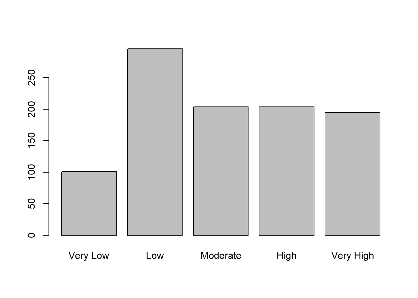
4.4.3.4 Deriving a new column from a calculation
movies <- mov[, c(2, 5, 7, 8, 11)]
movies$Rev.Run <- round(movies$Revenue/movies$Runtime, 2)
head(movies)
#>                     Title             Director Year Runtime
#> 1 Guardians of the Galaxy           James Gunn 2014     121
#> 2              Prometheus         Ridley Scott 2012     124
#> 3                   Split   M. Night Shyamalan 2016     117
#> 4                    Sing Christophe Lourdelet 2016     108
#> 5           Suicide Squad           David Ayer 2016     123
#> 6          The Great Wall          Yimou Zhang 2016     103
#>   Revenue Rev.Run
#> 1  333.13    2.75
#> 2  126.46    1.02
#> 3  138.12    1.18
#> 4  270.32    2.50
#> 5  325.02    2.64
#> 6   45.13    0.44
4.4.3.5 Updating a column
movies <- mov[,c(2, 5, 7, 9, 11, 12)]
movies$Director <- toupper(movies$Director)
movies$Title <- tolower(movies$Title)
head(movies)
#>                     Title             Director Year Rating
#> 1 guardians of the galaxy           JAMES GUNN 2014    8.1
#> 2              prometheus         RIDLEY SCOTT 2012    7.0
#> 3                   split   M. NIGHT SHYAMALAN 2016    7.3
#> 4                    sing CHRISTOPHE LOURDELET 2016    7.2
#> 5           suicide squad           DAVID AYER 2016    6.2
#> 6          the great wall          YIMOU ZHANG 2016    6.1
#>   Revenue Metascore
#> 1  333.13        76
#> 2  126.46        65
#> 3  138.12        62
#> 4  270.32        59
#> 5  325.02        40
#> 6   45.13        42
4.4.4 Sorting and ranking
4.4.4.1 Sorting a data frame
The order() function is used to sort a data frame. It takes a column and returns indices in ascending order. To reverse this, use decreasing = TRUE. Once the indices are sorted, they are used to index the data frame. The function order() also works on character columns as well and on multiple columns.
# sorting by revenue
movies <- mov[, c(2, 7, 11, 12)]
movies_ordered <- movies[order(movies$Revenue),]
head(movies_ordered)
#>                Title Year Revenue Metascore
#> 232 A Kind of Murder 2016    0.00        50
#> 28        Dead Awake 2016    0.01        NA
#> 69         Wakefield 2016    0.01        61
#> 322         Lovesong 2016    0.01        74
#> 678      Love, Rosie 2014    0.01        44
#> 962  Into the Forest 2015    0.01        59
tail(movies_ordered)
#>                              Title Year Revenue Metascore
#> 977                    Dark Places 2015      NA        39
#> 978                  Amateur Night 2016      NA        38
#> 979 It's Only the End of the World 2016      NA        48
#> 989                        Martyrs 2008      NA        89
#> 996           Secret in Their Eyes 2015      NA        45
#> 999                   Search Party 2014      NA        22

# sort decreasing
movies_ordered <- movies[order(movies$Revenue, decreasing = T),]
head(movies_ordered)
#>                                         Title Year Revenue
#> 51 Star Wars: Episode VII - The Force Awakens 2015  936.63
#> 88                                     Avatar 2009  760.51
#> 86                             Jurassic World 2015  652.18
#> 77                               The Avengers 2012  623.28
#> 55                            The Dark Knight 2008  533.32
#> 13                                  Rogue One 2016  532.17
#>    Metascore
#> 51        81
#> 88        83
#> 86        59
#> 77        69
#> 55        82
#> 13        65
tail(movies_ordered)
#>                              Title Year Revenue Metascore
#> 977                    Dark Places 2015      NA        39
#> 978                  Amateur Night 2016      NA        38
#> 979 It's Only the End of the World 2016      NA        48
#> 989                        Martyrs 2008      NA        89
#> 996           Secret in Their Eyes 2015      NA        45
#> 999                   Search Party 2014      NA        22

# sort decreasing using the negative sign
movies_ordered <- movies[order(-movies$Revenue),]
head(movies_ordered)
#>                                         Title Year Revenue
#> 51 Star Wars: Episode VII - The Force Awakens 2015  936.63
#> 88                                     Avatar 2009  760.51
#> 86                             Jurassic World 2015  652.18
#> 77                               The Avengers 2012  623.28
#> 55                            The Dark Knight 2008  533.32
#> 13                                  Rogue One 2016  532.17
#>    Metascore
#> 51        81
#> 88        83
#> 86        59
#> 77        69
#> 55        82
#> 13        65
tail(movies_ordered)
#>                              Title Year Revenue Metascore
#> 977                    Dark Places 2015      NA        39
#> 978                  Amateur Night 2016      NA        38
#> 979 It's Only the End of the World 2016      NA        48
#> 989                        Martyrs 2008      NA        89
#> 996           Secret in Their Eyes 2015      NA        45
#> 999                   Search Party 2014      NA        22
By default, NA values appear at the end of the sorted column, but this can be changed by setting na.last = FALSE so that they appear first.
# placing NA at the beginning
movies_ordered <- movies[order(movies$Revenue, na.last = FALSE),]
head(movies_ordered)
#>                      Title Year Revenue Metascore
#> 8                 Mindhorn 2016      NA        71
#> 23          Hounds of Love 2016      NA        72
#> 26         Paris pieds nus 2016      NA        NA
#> 40               5- 25- 77 2007      NA        NA
#> 43 Don't Fuck in the Woods 2016      NA        NA
#> 48                  Fallen 2016      NA        NA
tail(movies_ordered)
#>                                         Title Year Revenue
#> 13                                  Rogue One 2016  532.17
#> 55                            The Dark Knight 2008  533.32
#> 77                               The Avengers 2012  623.28
#> 86                             Jurassic World 2015  652.18
#> 88                                     Avatar 2009  760.51
#> 51 Star Wars: Episode VII - The Force Awakens 2015  936.63
#>    Metascore
#> 13        65
#> 55        82
#> 77        69
#> 86        59
#> 88        83
#> 51        81

# sorting on multiple columns
movies_ordered <- movies[order(movies$Metascore, movies$Revenue, decreasing = T),]
head(movies_ordered, 10)
#>                     Title Year Revenue Metascore
#> 657               Boyhood 2014   25.36       100
#> 42              Moonlight 2016   27.85        99
#> 231       Pan's Labyrinth 2006   37.62        98
#> 510               Gravity 2013  274.08        96
#> 490           Ratatouille 2007  206.44        96
#> 112      12 Years a Slave 2013   56.67        96
#> 22  Manchester by the Sea 2016   47.70        96
#> 325    The Social Network 2010   96.92        95
#> 407      Zero Dark Thirty 2012   95.72        95
#> 502                 Carol 2015    0.25        95
4.4.4.2 Ranking
The function rank() ranks column values. It does this in ascending order but can be reversed by placing a negative sign in front of the ranking column as there is no decreasing argument here as was the case with the order() function.
# returning ranks by revenue
rank(movies$Revenue)[1:10]
#>  [1] 841 678 702 819 839 419 724 873 182 623

# adding a rank to the data frame
movies <- mov[, c(2, 7, 11, 12)]
movies$Ranking <- rank(movies$Revenue)
head(movies)
#>                     Title Year Revenue Metascore Ranking
#> 1 Guardians of the Galaxy 2014  333.13        76     841
#> 2              Prometheus 2012  126.46        65     678
#> 3                   Split 2016  138.12        62     702
#> 4                    Sing 2016  270.32        59     819
#> 5           Suicide Squad 2016  325.02        40     839
#> 6          The Great Wall 2016   45.13        42     419

# sorting by rank
movies <- mov[, c(2, 7, 11, 12)]
movies$Ranking <- rank(movies$Revenue)
movies <- movies[order(movies$Ranking), ]
head(movies)
#>                Title Year Revenue Metascore Ranking
#> 232 A Kind of Murder 2016    0.00        50       1
#> 28        Dead Awake 2016    0.01        NA       4
#> 69         Wakefield 2016    0.01        61       4
#> 322         Lovesong 2016    0.01        74       4
#> 678      Love, Rosie 2014    0.01        44       4
#> 962  Into the Forest 2015    0.01        59       4

# placing NA values at the beginning
movies <- mov[, c(2, 7, 11, 12)]
movies$Ranking <- rank(movies$Revenue, na.last = F)
movies <- movies[order(movies$Ranking), ]
head(movies)
#>                      Title Year Revenue Metascore Ranking
#> 8                 Mindhorn 2016      NA        71       1
#> 23          Hounds of Love 2016      NA        72       2
#> 26         Paris pieds nus 2016      NA        NA       3
#> 40               5- 25- 77 2007      NA        NA       4
#> 43 Don't Fuck in the Woods 2016      NA        NA       5
#> 48                  Fallen 2016      NA        NA       6
There is no decreasing argument with rank(), hence our only chance of performing a decreasing rank is to use the negative sign.
# performing a decreasing rank
movies <- mov[, c(2, 7, 8, 11)]
movies$Ranking <- rank(-movies$Revenue)
movies <- movies[order(movies$Ranking), ]
head(movies)
#>                                         Title Year Runtime
#> 51 Star Wars: Episode VII - The Force Awakens 2015     136
#> 88                                     Avatar 2009     162
#> 86                             Jurassic World 2015     124
#> 77                               The Avengers 2012     143
#> 55                            The Dark Knight 2008     152
#> 13                                  Rogue One 2016     133
#>    Revenue Ranking
#> 51  936.63       1
#> 88  760.51       2
#> 86  652.18       3
#> 77  623.28       4
#> 55  533.32       5
#> 13  532.17       6
4.4.5 Splitting and Merging columns
4.4.5.1 Splitting columns
To split a data frame, we do the following
- select the column concerned and pass it to the function
strsplit()together with the string to split on. This will return a list - using the function
do.call('rbind', dfs)convert the list to a data frame - rename the columns of the new data frame
- finally using
cbind(), combine the new data frame to the original one
# Airports are ranked by travellers and experts based on various measures.
# https://www.kaggle.com/jonahmary17/airports

# reading data
busiestAirports <- read.table(file = "data/busiestAirports.csv",
                              header = T,
                              sep=",",
                              dec = ".",
                              quote = "\"")

busiestAirports <- busiestAirports[-c(1, 2, 3, 4, 8)]
head(busiestAirports, 3)
#>   code.iata.icao.                 location
#> 1        ATL/KATL         Atlanta, Georgia
#> 2        PEK/ZBAA Chaoyang-Shunyi, Beijing
#> 3        DXB/OMDB           Garhoud, Dubai
#>                country
#> 1        United States
#> 2                China
#> 3 United Arab Emirates

# splitting column
strsplit(busiestAirports$code.iata.icao.,'/')[1:3]
#> [[1]]
#> [1] "ATL"  "KATL"
#>
#> [[2]]
#> [1] "PEK"  "ZBAA"
#>
#> [[3]]
#> [1] "DXB"  "OMDB"

# converting to a data frame
iata_icao <-
data.frame(do.call('rbind', strsplit(busiestAirports$code.iata.icao., '/')))
head(iata_icao, 3)
#>    X1   X2
#> 1 ATL KATL
#> 2 PEK ZBAA
#> 3 DXB OMDB

# renaming columns
names(iata_icao) <- c('iata', 'icao')
head(iata_icao, 3)
#>   iata icao
#> 1  ATL KATL
#> 2  PEK ZBAA
#> 3  DXB OMDB

# combining both data frames
busiest_Airports <- cbind(busiestAirports[-1], iata_icao)
head(busiest_Airports)
#>                   location              country iata icao
#> 1         Atlanta, Georgia        United States  ATL KATL
#> 2 Chaoyang-Shunyi, Beijing                China  PEK ZBAA
#> 3           Garhoud, Dubai United Arab Emirates  DXB OMDB
#> 4  Los Angeles, California        United States  LAX KLAX
#> 5               Ota, Tokyo                Japan  HND RJTT
#> 6        Chicago, Illinois        United States  ORD KORD
4.4.5.2 Merging columns
The function paste() is used to merge columns.
# merging iata and icao into iata_icao
busiest_Airports$iata_icao <-
paste(busiest_Airports$iata, busiest_Airports$icao, sep = '-')
head(busiest_Airports)
#>                   location              country iata icao
#> 1         Atlanta, Georgia        United States  ATL KATL
#> 2 Chaoyang-Shunyi, Beijing                China  PEK ZBAA
#> 3           Garhoud, Dubai United Arab Emirates  DXB OMDB
#> 4  Los Angeles, California        United States  LAX KLAX
#> 5               Ota, Tokyo                Japan  HND RJTT
#> 6        Chicago, Illinois        United States  ORD KORD
#>   iata_icao
#> 1  ATL-KATL
#> 2  PEK-ZBAA
#> 3  DXB-OMDB
#> 4  LAX-KLAX
#> 5  HND-RJTT
#> 6  ORD-KORD
4.5 Selecting columns
The function subset() or [ is used to select columns.
head(gapminder_cp1250[, c(1, 3)])
#>       country year
#> 1 Afghanistan 1952
#> 2 Afghanistan 1957
#> 3 Afghanistan 1962
#> 4 Afghanistan 1967
#> 5 Afghanistan 1972
#> 6 Afghanistan 1977
head(gapminder_cp1250[, c("country", "gdpPercap")])
#>       country gdpPercap
#> 1 Afghanistan  779.4453
#> 2 Afghanistan  820.8530
#> 3 Afghanistan  853.1007
#> 4 Afghanistan  836.1971
#> 5 Afghanistan  739.9811
#> 6 Afghanistan  786.1134
head(subset(gapminder_cp1250, select = c("country", "gdpPercap")))
#>       country gdpPercap
#> 1 Afghanistan  779.4453
#> 2 Afghanistan  820.8530
#> 3 Afghanistan  853.1007
#> 4 Afghanistan  836.1971
#> 5 Afghanistan  739.9811
#> 6 Afghanistan  786.1134
4.6 Deleting columns
There is no special function to delete columns but [ and NULL can be used to drop unwanted columns.
str(gapminder_cp1250)
#> 'data.frame':    1704 obs. of  8 variables:
#>  $ country      : chr  "Afghanistan" "Afghanistan" "Afghanistan" "Afghanistan" ...
#>  $ continent    : chr  "Asia" "Asia" "Asia" "Asia" ...
#>  $ year         : int  1952 1957 1962 1967 1972 1977 1982 1987 1992 1997 ...
#>  $ lifeExp      : num  28.8 30.3 32 34 36.1 ...
#>  $ pop          : int  8425333 9240934 10267083 11537966 13079460 14880372 12881816 13867957 16317921 22227415 ...
#>  $ gdpPercap    : num  779 821 853 836 740 ...
#>  $ country_hun  : chr  "Afganisztán" "Afganisztán" "Afganisztán" "Afganisztán" ...
#>  $ continent_hun: chr  "Ázsia" "Ázsia" "Ázsia" "Ázsia" ...
gapminder_cp1250$pop <- NULL
str(gapminder_cp1250)
#> 'data.frame':    1704 obs. of  7 variables:
#>  $ country      : chr  "Afghanistan" "Afghanistan" "Afghanistan" "Afghanistan" ...
#>  $ continent    : chr  "Asia" "Asia" "Asia" "Asia" ...
#>  $ year         : int  1952 1957 1962 1967 1972 1977 1982 1987 1992 1997 ...
#>  $ lifeExp      : num  28.8 30.3 32 34 36.1 ...
#>  $ gdpPercap    : num  779 821 853 836 740 ...
#>  $ country_hun  : chr  "Afganisztán" "Afganisztán" "Afganisztán" "Afganisztán" ...
#>  $ continent_hun: chr  "Ázsia" "Ázsia" "Ázsia" "Ázsia" ...
gapminder_cp1250 <- gapminder_cp1250[, c(1, 2, 5, 6)]
str(gapminder_cp1250)
#> 'data.frame':    1704 obs. of  4 variables:
#>  $ country    : chr  "Afghanistan" "Afghanistan" "Afghanistan" "Afghanistan" ...
#>  $ continent  : chr  "Asia" "Asia" "Asia" "Asia" ...
#>  $ gdpPercap  : num  779 821 853 836 740 ...
#>  $ country_hun: chr  "Afganisztán" "Afganisztán" "Afganisztán" "Afganisztán" ...
4.7 Manipulating Rows
4.7.1 Renaming rows
After importing data, rows can be renamed by assigning new names to them.
rownames(gapminder_utf8)[1:6]
#> [1] "1" "2" "3" "4" "5" "6"
rownames(gapminder_utf8) <- paste0("RN-", 1:nrow(gapminder_utf8))
head(gapminder_utf8)
#>           orszag kontinens year lifeExp      pop gdpPercap
#> RN-1 Afghanistan      Asia 1952  28.801  8425333  779.4453
#> RN-2 Afghanistan      Asia 1957  30.332  9240934  820.8530
#> RN-3 Afghanistan      Asia 1962  31.997 10267083  853.1007
#> RN-4 Afghanistan      Asia 1967  34.020 11537966  836.1971
#> RN-5 Afghanistan      Asia 1972  36.088 13079460  739.9811
#> RN-6 Afghanistan      Asia 1977  38.438 14880372  786.1134
#>       orszag_hun kontinens_hun
#> RN-1 Afganisztán         Ázsia
#> RN-2 Afganisztán         Ázsia
#> RN-3 Afganisztán         Ázsia
#> RN-4 Afganisztán         Ázsia
#> RN-5 Afganisztán         Ázsia
#> RN-6 Afganisztán         Ázsia
rownames(gapminder_utf8) <- 1:nrow(gapminder_utf8) # reset row names
head(gapminder_utf8)
#>        orszag kontinens year lifeExp      pop gdpPercap
#> 1 Afghanistan      Asia 1952  28.801  8425333  779.4453
#> 2 Afghanistan      Asia 1957  30.332  9240934  820.8530
#> 3 Afghanistan      Asia 1962  31.997 10267083  853.1007
#> 4 Afghanistan      Asia 1967  34.020 11537966  836.1971
#> 5 Afghanistan      Asia 1972  36.088 13079460  739.9811
#> 6 Afghanistan      Asia 1977  38.438 14880372  786.1134
#>    orszag_hun kontinens_hun
#> 1 Afganisztán         Ázsia
#> 2 Afganisztán         Ázsia
#> 3 Afganisztán         Ázsia
#> 4 Afganisztán         Ázsia
#> 5 Afganisztán         Ázsia
#> 6 Afganisztán         Ázsia
4.7.2 Adding rows
4.7.2.1 Adding rows by assignment
movies <- mov[, c(2, 5, 7, 9, 11, 12)]
tail(movies, 3)
#>                       Title         Director Year Rating
#> 998  Step Up 2: The Streets       Jon M. Chu 2008    6.2
#> 999            Search Party   Scot Armstrong 2014    5.6
#> 1000             Nine Lives Barry Sonnenfeld 2016    5.3
#>      Revenue Metascore
#> 998    58.01        50
#> 999       NA        22
#> 1000   19.64        11

# inserting rows
movies[1001,] <- c("the big g", "goro lovic", 2015, 9.9, 1000, 100)
movies[1002,] <- c("luv of my life", "nema lovic", 2016, 7.9, 150, 65)
movies[1003,] <- c("everyday", "goro lovic", 2014, 4.4, 170, 40)
tail(movies)
#>                       Title         Director Year Rating
#> 998  Step Up 2: The Streets       Jon M. Chu 2008    6.2
#> 999            Search Party   Scot Armstrong 2014    5.6
#> 1000             Nine Lives Barry Sonnenfeld 2016    5.3
#> 1001              the big g       goro lovic 2015    9.9
#> 1002         luv of my life       nema lovic 2016    7.9
#> 1003               everyday       goro lovic 2014    4.4
#>      Revenue Metascore
#> 998    58.01        50
#> 999     <NA>        22
#> 1000   19.64        11
#> 1001    1000       100
#> 1002     150        65
#> 1003     170        40

# using nrow
movies <- mov[, c(2, 5, 7, 9, 11, 12)]
movies[nrow(movies) + 1,] <- c("the big g", "goro lovic", 2015, 9.9, 1000, 100)
movies[nrow(movies) + 1,] <- c("luv of my life", "nema lovic", 2016, 7.9, 150, 65)
movies[nrow(movies) + 1,] <- c("everyday", "goro lovic", 2014, 4.4, 170, 40)
tail(movies)
#>                       Title         Director Year Rating
#> 998  Step Up 2: The Streets       Jon M. Chu 2008    6.2
#> 999            Search Party   Scot Armstrong 2014    5.6
#> 1000             Nine Lives Barry Sonnenfeld 2016    5.3
#> 1001              the big g       goro lovic 2015    9.9
#> 1002         luv of my life       nema lovic 2016    7.9
#> 1003               everyday       goro lovic 2014    4.4
#>      Revenue Metascore
#> 998    58.01        50
#> 999     <NA>        22
#> 1000   19.64        11
#> 1001    1000       100
#> 1002     150        65
#> 1003     170        40
The function rbind() can combine both a list or a vector to a data frame. Generally, avoid using vectors as they may change the data type of the data frame.
4.7.2.2 Adding rows using rbind()
# binding a list to a data frame
movies <- mov[, c(2, 5, 7, 9, 11, 12)]
movies <- rbind(movies, list("the big g", "goro lovic", 2015, 9.9, 1000, 100))
movies <- rbind(movies, list("luv of my life", "nema lovic", 2016, 7.9, 150, 65))
movies <- rbind(movies, list("everyday", "goro lovic", 2014, 4.4, 170, 40))
tail(movies)
#>                       Title         Director Year Rating
#> 998  Step Up 2: The Streets       Jon M. Chu 2008    6.2
#> 999            Search Party   Scot Armstrong 2014    5.6
#> 1000             Nine Lives Barry Sonnenfeld 2016    5.3
#> 1001              the big g       goro lovic 2015    9.9
#> 1002         luv of my life       nema lovic 2016    7.9
#> 1003               everyday       goro lovic 2014    4.4
#>      Revenue Metascore
#> 998    58.01        50
#> 999       NA        22
#> 1000   19.64        11
#> 1001 1000.00       100
#> 1002  150.00        65
#> 1003  170.00        40

movies <- mov[, c(2, 5, 7, 9, 11, 12)]
sapply(movies, class)
#>       Title    Director        Year      Rating     Revenue
#> "character" "character"   "integer"   "numeric"   "numeric"
#>   Metascore
#>   "integer"

# using a vector
movies <- rbind(movies, c("the big g", "goro lovic", 2015, 9.9, 1000, 100))
sapply(movies, class)
#>       Title    Director        Year      Rating     Revenue
#> "character" "character" "character" "character" "character"
#>   Metascore
#> "character"
4.7.2.3 Adding rows using do.call()
The function do.call('rbind', dfs) combines a list of data frames, list, and vectors. Again, avoid using vectors as they may change the data type of the data frames.
movies <- subset(mov, select = c(2, 5, 7, 9, 11, 12))
movies <- do.call('rbind', list(movies,
                                list("the big g", "goro lovic", 2015, 9.9, 1000, 100),
                                list("luv of my life", "nema lovic", 2016, 7.9, 150, 65),
                                list("everyday", "goro lovic", 2014, 4.4, 170, 40)))
tail(movies)
#>                       Title         Director Year Rating
#> 998  Step Up 2: The Streets       Jon M. Chu 2008    6.2
#> 999            Search Party   Scot Armstrong 2014    5.6
#> 1000             Nine Lives Barry Sonnenfeld 2016    5.3
#> 1001              the big g       goro lovic 2015    9.9
#> 1002         luv of my life       nema lovic 2016    7.9
#> 1003               everyday       goro lovic 2014    4.4
#>      Revenue Metascore
#> 998    58.01        50
#> 999       NA        22
#> 1000   19.64        11
#> 1001 1000.00       100
#> 1002  150.00        65
#> 1003  170.00        40
4.7.3 Updating rows of data
To update a row, we simply select it and give it a new list of values. Vectors can be used also but should be avoided as they may change the data type of the data frame.
movies <- mov[, c(1, 2, 5, 7, 9, 11, 12)]
movies[6,]
#>   Rank          Title    Director Year Rating Revenue
#> 6    6 The Great Wall Yimou Zhang 2016    6.1   45.13
#>   Metascore
#> 6        42

# updating a row by indexing
movies[6,] <- list(6, 'I am coming home', 'goro lovic', 2020, 9.8, 850, 85)
movies[6,]
#>   Rank            Title   Director Year Rating Revenue
#> 6    6 I am coming home goro lovic 2020    9.8     850
#>   Metascore
#> 6        85

# updating a row by filtering
movies <- mov[, c(1, 2, 5, 7, 9, 11, 12)]
movies[movies$Rank == 6,] <- list(6, 'I am coming home', 'goro lovic', 2020, 9.8, 850, 85)
movies[movies$Rank == 6,]
#>   Rank            Title   Director Year Rating Revenue
#> 6    6 I am coming home goro lovic 2020    9.8     850
#>   Metascore
#> 6        85
4.7.4 Updating a single value
To update a single value, we select it through subsetting and assign it a new value.
movies <- mov[, c(1, 2, 5, 7, 9, 11, 12)]
movies[movies$Director == 'Christopher Nolan',]
#>     Rank                 Title          Director Year
#> 37    37          Interstellar Christopher Nolan 2014
#> 55    55       The Dark Knight Christopher Nolan 2008
#> 65    65          The Prestige Christopher Nolan 2006
#> 81    81             Inception Christopher Nolan 2010
#> 125  125 The Dark Knight Rises Christopher Nolan 2012
#>     Rating Revenue Metascore
#> 37     8.6  187.99        74
#> 55     9.0  533.32        82
#> 65     8.5   53.08        66
#> 81     8.8  292.57        74
#> 125    8.5  448.13        78

# changing from 'Christopher Nolan' to 'C Nolan'
movies[movies$Director == 'Christopher Nolan', 'Director'] <- 'C Nolan'
movies[c(37, 55, 65, 81, 125),]
#>     Rank                 Title Director Year Rating Revenue
#> 37    37          Interstellar  C Nolan 2014    8.6  187.99
#> 55    55       The Dark Knight  C Nolan 2008    9.0  533.32
#> 65    65          The Prestige  C Nolan 2006    8.5   53.08
#> 81    81             Inception  C Nolan 2010    8.8  292.57
#> 125  125 The Dark Knight Rises  C Nolan 2012    8.5  448.13
#>     Metascore
#> 37         74
#> 55         82
#> 65         66
#> 81         74
#> 125        78
4.7.5 Randomly selecting rows
To select a random sample of rows, we use the function sample().
# selecting 10 random rows
movies <- mov[, c(2, 7, 11, 12)]
movies[sample(x = nrow(movies), size = 10), ]
#>                    Title Year Revenue Metascore
#> 535      A Quiet Passion 2016    1.08        77
#> 471    American Gangster 2007  130.13        76
#> 728      The Illusionist 2006   39.83        68
#> 789 Hotel Transylvania 2 2015  169.69        44
#> 978        Amateur Night 2016      NA        38
#> 275            Ballerina 2016      NA        NA
#> 905              RoboCop 2014   58.61        52
#> 723            Grown Ups 2010  162.00        30
#> 958         End of Watch 2012   40.98        68
#> 211          San Andreas 2015  155.18        43
4.7.6 Filtering rows
The function subset() or [ is used to filter rows.
head(gapminder_cp1250[gapminder_cp1250$continent == "Europe", c("country", "gdpPercap", "continent")])
#>    country gdpPercap continent
#> 13 Albania  1601.056    Europe
#> 14 Albania  1942.284    Europe
#> 15 Albania  2312.889    Europe
#> 16 Albania  2760.197    Europe
#> 17 Albania  3313.422    Europe
#> 18 Albania  3533.004    Europe
gapminder_cp1250[gapminder_cp1250$continent == "Europe" & gapminder_cp1250$gdpPercap > 2000 & gapminder_cp1250$gdpPercap < 4000, c("country", "gdpPercap", "continent")]
#>                     country gdpPercap continent
#> 15                  Albania  2312.889    Europe
#> 16                  Albania  2760.197    Europe
#> 17                  Albania  3313.422    Europe
#> 18                  Albania  3533.004    Europe
#> 19                  Albania  3630.881    Europe
#> 20                  Albania  3738.933    Europe
#> 21                  Albania  2497.438    Europe
#> 22                  Albania  3193.055    Europe
#> 148  Bosnia and Herzegovina  2172.352    Europe
#> 149  Bosnia and Herzegovina  2860.170    Europe
#> 150  Bosnia and Herzegovina  3528.481    Europe
#> 153  Bosnia and Herzegovina  2546.781    Europe
#> 181                Bulgaria  2444.287    Europe
#> 182                Bulgaria  3008.671    Europe
#> 373                 Croatia  3119.237    Europe
#> 589                  Greece  3530.690    Europe
#> 1009             Montenegro  2647.586    Europe
#> 1010             Montenegro  3682.260    Europe
#> 1237               Portugal  3068.320    Europe
#> 1238               Portugal  3774.572    Europe
#> 1273                Romania  3144.613    Europe
#> 1274                Romania  3943.370    Europe
#> 1333                 Serbia  3581.459    Europe
#> 1417                  Spain  3834.035    Europe
#> 1574                 Turkey  2218.754    Europe
#> 1575                 Turkey  2322.870    Europe
#> 1576                 Turkey  2826.356    Europe
#> 1577                 Turkey  3450.696    Europe
subset(gapminder_cp1250,
       subset =  continent == "Europe" & gdpPercap > 2000 & gdpPercap < 4000,
       select = c("country", "gdpPercap", "continent"))
#>                     country gdpPercap continent
#> 15                  Albania  2312.889    Europe
#> 16                  Albania  2760.197    Europe
#> 17                  Albania  3313.422    Europe
#> 18                  Albania  3533.004    Europe
#> 19                  Albania  3630.881    Europe
#> 20                  Albania  3738.933    Europe
#> 21                  Albania  2497.438    Europe
#> 22                  Albania  3193.055    Europe
#> 148  Bosnia and Herzegovina  2172.352    Europe
#> 149  Bosnia and Herzegovina  2860.170    Europe
#> 150  Bosnia and Herzegovina  3528.481    Europe
#> 153  Bosnia and Herzegovina  2546.781    Europe
#> 181                Bulgaria  2444.287    Europe
#> 182                Bulgaria  3008.671    Europe
#> 373                 Croatia  3119.237    Europe
#> 589                  Greece  3530.690    Europe
#> 1009             Montenegro  2647.586    Europe
#> 1010             Montenegro  3682.260    Europe
#> 1237               Portugal  3068.320    Europe
#> 1238               Portugal  3774.572    Europe
#> 1273                Romania  3144.613    Europe
#> 1274                Romania  3943.370    Europe
#> 1333                 Serbia  3581.459    Europe
#> 1417                  Spain  3834.035    Europe
#> 1574                 Turkey  2218.754    Europe
#> 1575                 Turkey  2322.870    Europe
#> 1576                 Turkey  2826.356    Europe
#> 1577 Turkey 3450.696 Europe4.8 SQL like joins
At the most basic level there are four types of SQL joins:
- Inner join: which returns only rows matched in both data frames
- Left join (left outer join): which returns all rows found in the left data frame irrespective of whether they are matched to rows in the right data frame. If rows do not match values in the right data frames, NA values are returned instead.
- Right join (right outer join): which is the reverse of the left join, that is it returns all rows found on the right data frame irrespective of whether they are matched on the left data frame.
- Outer join (full outer join): returns all rows from both data frames irrespective of whether they are matched or not
4.8.1 Inner join
# preparing data
employees <- data.frame(
  name = c('john', 'mary', 'david', 'paul', 'susan', 'cynthia', 'Joss', 'dennis'),
  age = c(45, 55, 35, 58, 40, 30, 39, 25),
  gender = c('m', 'f', 'm', 'm', 'f', 'f', 'm', 'm'),
  salary =c(40000, 50000, 35000, 25000, 48000, 32000, 20000, 45000),
  department = c('commercial', 'production', NA, 'human resources',
                 'commercial', 'commercial', 'production', NA))
employees
#>      name age gender salary      department
#> 1    john  45      m  40000      commercial
#> 2    mary  55      f  50000      production
#> 3   david  35      m  35000            <NA>
#> 4    paul  58      m  25000 human resources
#> 5   susan  40      f  48000      commercial
#> 6 cynthia  30      f  32000      commercial
#> 7    Joss  39      m  20000      production
#> 8  dennis  25      m  45000            <NA>
departments <- data.frame(
  department = c('commercial', 'human resources', 'production', 'finance', 'maintenance'),
  location = c('washington', 'london', 'paris', 'dubai', 'dublin'))
departments
#>        department   location
#> 1      commercial washington
#> 2 human resources     london
#> 3      production      paris
#> 4         finance      dubai
#> 5     maintenance     dublin

# returns only rows that are matched in both data frames
merge(employees, departments, by = "department")
#>        department    name age gender salary   location
#> 1      commercial    john  45      m  40000 washington
#> 2      commercial   susan  40      f  48000 washington
#> 3      commercial cynthia  30      f  32000 washington
#> 4 human resources    paul  58      m  25000     london
#> 5      production    mary  55      f  50000      paris
#> 6      production    Joss  39      m  20000      paris
4.8.2 Left join
To perform a left join, the argument all.x = TRUE is used.
# returns all the values of the left data frame
merge(employees, departments, by = "department", all.x = TRUE)
#>        department    name age gender salary   location
#> 1      commercial    john  45      m  40000 washington
#> 2      commercial   susan  40      f  48000 washington
#> 3      commercial cynthia  30      f  32000 washington
#> 4 human resources    paul  58      m  25000     london
#> 5      production    mary  55      f  50000      paris
#> 6      production    Joss  39      m  20000      paris
#> 7            <NA>   david  35      m  35000       <NA>
#> 8            <NA>  dennis  25      m  45000       <NA>
4.8.3 Right join
To perform a right join, the argument all.y = TRUE is used.
# returns all the values of the right table
merge(employees, departments, by = "department", all.y = TRUE)
#>        department    name age gender salary   location
#> 1      commercial    john  45      m  40000 washington
#> 2      commercial   susan  40      f  48000 washington
#> 3      commercial cynthia  30      f  32000 washington
#> 4         finance    <NA>  NA   <NA>     NA      dubai
#> 5 human resources    paul  58      m  25000     london
#> 6     maintenance    <NA>  NA   <NA>     NA     dublin
#> 7      production    mary  55      f  50000      paris
#> 8      production    Joss  39      m  20000      paris

# reversing the tables in the right join produces the same results as the left join
merge(departments, employees , by = "department", all.y = TRUE)
#>        department   location    name age gender salary
#> 1      commercial washington    john  45      m  40000
#> 2      commercial washington   susan  40      f  48000
#> 3      commercial washington cynthia  30      f  32000
#> 4 human resources     london    paul  58      m  25000
#> 5      production      paris    mary  55      f  50000
#> 6      production      paris    Joss  39      m  20000
#> 7            <NA>       <NA>   david  35      m  35000
#> 8            <NA>       <NA>  dennis  25      m  45000
4.8.4 Full outer join
To perform a full join, the argument all = TRUE is used.
# returns all rows
merge(employees, departments, by = "department", all = TRUE)
#>         department    name age gender salary   location
#> 1       commercial    john  45      m  40000 washington
#> 2       commercial   susan  40      f  48000 washington
#> 3       commercial cynthia  30      f  32000 washington
#> 4          finance    <NA>  NA   <NA>     NA      dubai
#> 5  human resources    paul  58      m  25000     london
#> 6      maintenance    <NA>  NA   <NA>     NA     dublin
#> 7       production    mary  55      f  50000      paris
#> 8       production    Joss  39      m  20000      paris
#> 9             <NA>   david  35      m  35000       <NA>
#> 10            <NA>  dennis  25      m  45000       <NA>
4.8.5 Joining data frames with different column names
The arguments by.x= and by.y= are used to declare the joining column(s) for the left and right data frames, respectively.
# recreating the employee table
employees <- data.frame(
  name = c('john', 'mary', 'david', 'paul', 'susan', 'cynthia', 'Joss', 'dennis'),
  age = c(45, 55, 35, 58, 40, 30, 39, 25),
  gender = c('m', 'f', 'm', 'm', 'f', 'f', 'm', 'm'),
  salary =c(40000, 50000, 35000, 25000, 48000, 32000, 20000, 45000),
  dep_name = c('commercial', 'production', NA, 'human resources', 'commercial',
               'commercial', 'production', NA))
head(employees, 2)
#>   name age gender salary   dep_name
#> 1 john  45      m  40000 commercial
#> 2 mary  55      f  50000 production
head(departments, 2)
#>        department   location
#> 1      commercial washington
#> 2 human resources     london

# joining on columns with different names
merge(employees, departments, by.x = 'dep_name', by.y = 'department')
#>          dep_name    name age gender salary   location
#> 1      commercial    john  45      m  40000 washington
#> 2      commercial   susan  40      f  48000 washington
#> 3      commercial cynthia  30      f  32000 washington
#> 4 human resources    paul  58      m  25000     london
#> 5      production    mary  55      f  50000      paris
#> 6      production    Joss  39      m  20000      paris
4.8.6 Joining data frames on one more than one joining column
If both data frames contain two or more columns with the same name, merge() will try performing the join using those column names.
# recreating the employees table
employees <- data.frame(
  name = c('john', 'mary', 'david', 'paul', 'susan', 'cynthia', 'Joss', 'dennis'),
  age = c(45, 55, 35, 58, 40, 30, 39, 25),
  gender = c('m', 'f', 'm', 'm', 'f', 'f', 'm', 'm'),
  salary =c(40000, 50000, 35000, 25000, 48000, 32000, 20000, 45000),
  department = c('commercial', 'production', NA, 'human resources', 'commercial',
                 'commercial', 'production', NA),
  subdepartment = c('marketing', 'production', NA, 'human resources', 'sales', 'sales',
                    'production', NA))
head(employees, 2)
#>   name age gender salary department subdepartment
#> 1 john  45      m  40000 commercial     marketing
#> 2 mary  55      f  50000 production    production

# creating the departments? table
departments <- data.frame(
  department = c('commercial', 'commercial', 'human resources', 'production', 'finance',
                 'finance', 'maintenance'),
  subdepartment = c('marketing', 'sales', 'human resources', 'production', 'finance',
                    'accounting', 'maintenance'),
  location = c('washington', 'washington', 'london', 'paris', 'dubai', 'dubai', 'dublin')
)
head(departments, 2)
#>   department subdepartment   location
#> 1 commercial     marketing washington
#> 2 commercial         sales washington

# because they both contain the same name, the join is performed automatically
merge(employees, departments)
#>        department   subdepartment    name age gender salary
#> 1      commercial       marketing    john  45      m  40000
#> 2      commercial           sales   susan  40      f  48000
#> 3      commercial           sales cynthia  30      f  32000
#> 4 human resources human resources    paul  58      m  25000
#> 5      production      production    mary  55      f  50000
#> 6      production      production    Joss  39      m  20000
#>     location
#> 1 washington
#> 2 washington
#> 3 washington
#> 4     london
#> 5      paris
#> 6      paris
If the data frames had columns of different names to join on, we would have used the arguments by.x= and by.y= to specify them as below.
# specifying joining columns
merge(employees, departments,
      by.x = c('department', 'subdepartment'),
      by.y =c('department', 'subdepartment'))
#>        department   subdepartment    name age gender salary
#> 1      commercial       marketing    john  45      m  40000
#> 2      commercial           sales   susan  40      f  48000
#> 3      commercial           sales cynthia  30      f  32000
#> 4 human resources human resources    paul  58      m  25000
#> 5      production      production    mary  55      f  50000
#> 6      production      production    Joss  39      m  20000
#>     location
#> 1 washington
#> 2 washington
#> 3 washington
#> 4     london
#> 5      paris
#> 6      paris
4.9 Aggregating and grouping data
The function aggregate() groups a data frame by a specific column value and performs summarization (sum, mean, median, length, min, max, etc.) based on those groups. It does a split-apply-combine, that is splitting a data frame by groups (category) after which it applies a calculation on each group and finally combines the results back together to create a single data frame which is presented as output.
# preparing data
gapminder_xlsx_2007 <- gapminder_xlsx[gapminder_xlsx$year == 2007, ]
head(gapminder_xlsx_2007)
#>        country continent year lifeExp      pop  gdpPercap
#> 12 Afghanistan      Asia 2007  43.828 31889923   974.5803
#> 24     Albania    Europe 2007  76.423  3600523  5937.0295
#> 36     Algeria    Africa 2007  72.301 33333216  6223.3675
#> 48      Angola    Africa 2007  42.731 12420476  4797.2313
#> 60   Argentina  Americas 2007  75.320 40301927 12779.3796
#> 72   Australia   Oceania 2007  81.235 20434176 34435.3674
#>    country_hun continent_hun
#> 12 Afganisztán         Ázsia
#> 24     Albánia        Európa
#> 36     Algéria        Afrika
#> 48      Angola        Afrika
#> 60   Argentína       Amerika
#> 72  Ausztrália       Óceánia

# population by continent
aggregate(pop ~ continent, gapminder_xlsx_2007, sum)
#>   continent        pop
#> 1    Africa  929539692
#> 2  Americas  898871184
#> 3      Asia 3811953827
#> 4    Europe  586098529
#> 5   Oceania   24549947
aggregate(pop ~ continent, gapminder_xlsx_2007, mean)
#>   continent       pop
#> 1    Africa  17875763
#> 2  Americas  35954847
#> 3      Asia 115513752
#> 4    Europe  19536618
#> 5   Oceania  12274974
The aggregate() function above, groups the data frame gapminder_xlsx_2007 by continent, after which it applies sum to each group.
Rather than filtering the data before passing it to the aggregate() function, we can filter the data directly inside aggregate() using the subset= argument.
# filtering with the subset argument
aggregate(pop ~ continent, gapminder_xlsx,
          subset = year == 2007,
          sum)
#>   continent        pop
#> 1    Africa  929539692
#> 2  Americas  898871184
#> 3      Asia 3811953827
#> 4    Europe  586098529
#> 5   Oceania   24549947
The + sign is used to group by more than one categorical column.
# pop by continent and year
aggregate(pop ~ continent + year,
          gapminder_xlsx,
          subset = year %in% c(1987, 2007),
          sum)
#>    continent year        pop
#> 1     Africa 1987  574834110
#> 2   Americas 1987  682753971
#> 3       Asia 1987 2871220762
#> 4     Europe 1987  543094160
#> 5    Oceania 1987   19574415
#> 6     Africa 2007  929539692
#> 7   Americas 2007  898871184
#> 8       Asia 2007 3811953827
#> 9     Europe 2007  586098529
#> 10   Oceania 2007   24549947
# using mean
aggregate(pop ~ continent + year,
          gapminder_xlsx,
          subset = year %in% c(1987, 2007),
          mean)
#>    continent year       pop
#> 1     Africa 1987  11054502
#> 2   Americas 1987  27310159
#> 3       Asia 1987  87006690
#> 4     Europe 1987  18103139
#> 5    Oceania 1987   9787208
#> 6     Africa 2007  17875763
#> 7   Americas 2007  35954847
#> 8       Asia 2007 115513752
#> 9     Europe 2007  19536618
#> 10   Oceania 2007  12274974
The function cbind() is used to aggregate on multiple columns, the only problem is that only one summarisation function can be used.
# aggregating on two numeric columns (lifeExp and gdpPercap)
aggregate(cbind(lifeExp, gdpPercap) ~ continent + year,
          gapminder_xlsx,
          subset = year %in% c(1987, 2007),
          mean)
#>    continent year  lifeExp gdpPercap
#> 1     Africa 1987 53.34479  2282.669
#> 2   Americas 1987 68.09072  7793.400
#> 3       Asia 1987 64.85118  7608.227
#> 4     Europe 1987 73.64217 17214.311
#> 5    Oceania 1987 75.32000 20448.040
#> 6     Africa 2007 54.80604  3089.033
#> 7   Americas 2007 73.60812 11003.032
#> 8       Asia 2007 70.72848 12473.027
#> 9     Europe 2007 77.64860 25054.482
#> 10   Oceania 2007 80.71950 29810.188
# rounding with customized function
aggregate(cbind(lifeExp, gdpPercap) ~ continent + year,
          gapminder_xlsx,
          subset = year %in% c(1987, 2007),
          function(x){round(mean(x), 1)})
#>    continent year lifeExp gdpPercap
#> 1     Africa 1987    53.3    2282.7
#> 2   Americas 1987    68.1    7793.4
#> 3       Asia 1987    64.9    7608.2
#> 4     Europe 1987    73.6   17214.3
#> 5    Oceania 1987    75.3   20448.0
#> 6     Africa 2007    54.8    3089.0
#> 7   Americas 2007    73.6   11003.0
#> 8       Asia 2007    70.7   12473.0
#> 9     Europe 2007    77.6   25054.5
#> 10   Oceania 2007    80.7   29810.2
4.10 Pivoting and unpivoting data
Tabular data exist in two forms: long and wide. The wide form is ideal for reporting while the long form is ideal for the computer. Most often, when performing data analysis, data in the wide form has to be converted to the long form (unpivoting) while when preparing reports, data in the long has to be converted to the wide form (pivoting).
wide data
| Person | Age | Weight | Height |
|---|---|---|---|
| Bob | 32 | 168 | 180 |
| Alice | 24 | 150 | 175 |
| Steve | 64 | 144 | 165 |
long data
| Person | Variable | Value |
|---|---|---|
| Bob | Age | 32 |
| Bob | Weight | 168 |
| Bob | Height | 180 |
| Alice | Age | 24 |
| Alice | Weight | 150 |
| Alice | Height | 175 |
| Steve | Age | 64 |
| Steve | Weight | 144 |
| Steve | Height | 165 |
4.10.1 Pivoting
Pivoting converts data frame rows to columns.
4.10.1.1 Pivoting using the reshape package
The reshape package is a package created for restructuring and aggregating data using just two functions: melt() and cast().
The function cast() pivots data while melt() unpivots data.
# preparing long data
dt <- aggregate(cbind(lifeExp, gdpPercap) ~ continent + year,
                gapminder_xlsx,
                subset = year >= 1987,
                mean)
head(dt,3)
#>   continent year  lifeExp gdpPercap
#> 1    Africa 1987 53.34479  2282.669
#> 2  Americas 1987 68.09072  7793.400
#> 3      Asia 1987 64.85118  7608.227
tail(dt,3)
#>    continent year  lifeExp gdpPercap
#> 23      Asia 2007 70.72848  12473.03
#> 24    Europe 2007 77.64860  25054.48
#> 25   Oceania 2007 80.71950  29810.19

library(reshape)
# converting from long to wide
cast(data = dt,
     formula = continent ~ year,
     value = 'lifeExp')
#>   continent     1987     1992     1997     2002     2007
#> 1    Africa 53.34479 53.62958 53.59827 53.32523 54.80604
#> 2  Americas 68.09072 69.56836 71.15048 72.42204 73.60812
#> 3      Asia 64.85118 66.53721 68.02052 69.23388 70.72848
#> 4    Europe 73.64217 74.44010 75.50517 76.70060 77.64860
#> 5   Oceania 75.32000 76.94500 78.19000 79.74000 80.71950
The function cast() can perform aggregation through the fun.aggregate= argument and filtering through the subset argument.
# summarization
cast(data = gapminder_xlsx_2007,
     formula = continent ~ year,
     value = 'pop',
     fun.aggregate = sum)
#>   continent       2007
#> 1    Africa  929539692
#> 2  Americas  898871184
#> 3      Asia 3811953827
#> 4    Europe  586098529
#> 5   Oceania   24549947

# filtering with subset
cast(data = gapminder_xlsx,
     continent ~ year,
     subset = year >= 1987,
     value = 'lifeExp',
     fun.aggregate = mean)
#>   continent     1987     1992     1997     2002     2007
#> 1    Africa 53.34479 53.62958 53.59827 53.32523 54.80604
#> 2  Americas 68.09072 69.56836 71.15048 72.42204 73.60812
#> 3      Asia 64.85118 66.53721 68.02052 69.23388 70.72848
#> 4    Europe 73.64217 74.44010 75.50517 76.70060 77.64860
#> 5   Oceania 75.32000 76.94500 78.19000 79.74000 80.71950

# rounding numbers
cast(data = gapminder_xlsx,
     continent ~ year,
     subset = year >= 1987,
     value = 'lifeExp',
     fun.aggregate = function(x)round(mean(x), 1))
#>   continent 1987 1992 1997 2002 2007
#> 1    Africa 53.3 53.6 53.6 53.3 54.8
#> 2  Americas 68.1 69.6 71.2 72.4 73.6
#> 3      Asia 64.9 66.5 68.0 69.2 70.7
#> 4    Europe 73.6 74.4 75.5 76.7 77.6
#> 5   Oceania 75.3 76.9 78.2 79.7 80.7

# population by year by continent
cast(data = gapminder_xlsx,
     year ~ continent,
     subset = year >= 1987,
     value = 'pop',
     fun.aggregate = sum)
#>   year    Africa  Americas       Asia    Europe  Oceania
#> 1 1987 574834110 682753971 2871220762 543094160 19574415
#> 2 1992 659081517 739274104 3133292191 558142797 20919651
#> 3 1997 743832984 796900410 3383285500 568944148 22241430
#> 4 2002 833723916 849772762 3601802203 578223869 23454829
#> 5 2007 929539692 898871184 3811953827 586098529 24549947
4.10.1.2 Pivoting using the reshape2 package
The reshape2 package is a reboot of the reshape package.
The function acast() and dcast() are used to pivot data with the former returning a matrix while the later a data frame.
dt_wide <- reshape2::acast(data = dt,
                           formula = continent ~ year,
                           value.var = 'lifeExp')
dt_wide
#>              1987     1992     1997     2002     2007
#> Africa   53.34479 53.62958 53.59827 53.32523 54.80604
#> Americas 68.09072 69.56836 71.15048 72.42204 73.60812
#> Asia     64.85118 66.53721 68.02052 69.23388 70.72848
#> Europe   73.64217 74.44010 75.50517 76.70060 77.64860
#> Oceania  75.32000 76.94500 78.19000 79.74000 80.71950
class(dt_wide)
#> [1] "matrix" "array"

dt_wide <- reshape2::dcast(data = dt,
                           formula = continent ~ year,
                           value.var = 'lifeExp')
dt_wide
#>   continent     1987     1992     1997     2002     2007
#> 1    Africa 53.34479 53.62958 53.59827 53.32523 54.80604
#> 2  Americas 68.09072 69.56836 71.15048 72.42204 73.60812
#> 3      Asia 64.85118 66.53721 68.02052 69.23388 70.72848
#> 4    Europe 73.64217 74.44010 75.50517 76.70060 77.64860
#> 5   Oceania 75.32000 76.94500 78.19000 79.74000 80.71950
class(dt_wide)
#> [1] "data.frame"

# filtering by year
reshape2::dcast(data = gapminder_xlsx[gapminder_xlsx$year >= 1987,],
                formula = continent ~ year,
                value.var = 'lifeExp',
                fun.aggregate = function(x)round(mean(x), 1))
#>   continent 1987 1992 1997 2002 2007
#> 1    Africa 53.3 53.6 53.6 53.3 54.8
#> 2  Americas 68.1 69.6 71.2 72.4 73.6
#> 3      Asia 64.9 66.5 68.0 69.2 70.7
#> 4    Europe 73.6 74.4 75.5 76.7 77.6
#> 5   Oceania 75.3 76.9 78.2 79.7 80.7
4.10.2 Unpivoting
Unpivoting converts data frame columns to rows.
The function melt() is used to unpivot data. It accepts the following:
-
id.vars=: columns not to be moved -
measure.vars=: columns to move to rows
but can guess both by default.
It is the same function name for reshape and reshape2.
dt_long <- melt(dt_wide)
head(dt_long)
#>   continent variable    value
#> 1    Africa     1987 53.34479
#> 2  Americas     1987 68.09072
#> 3      Asia     1987 64.85118
#> 4    Europe     1987 73.64217
#> 5   Oceania     1987 75.32000
#> 6    Africa     1992 53.62958

dt_long <- reshape2::melt(dt_wide)
head(dt_long)
#>   continent variable    value
#> 1    Africa     1987 53.34479
#> 2  Americas     1987 68.09072
#> 3      Asia     1987 64.85118
#> 4    Europe     1987 73.64217
#> 5   Oceania     1987 75.32000
#> 6    Africa     1992 53.62958
With the argument measure.vars=, we can filter the data frame.
# adding a variable name and filtering data
dt_long <- melt(dt_wide,
                id.vars = 'continent',
                variable_name = 'Year',
                measure.vars = c('1997', '2002', '2007'))
head(dt_long)
#>   continent Year    value
#> 1    Africa 1997 53.59827
#> 2  Americas 1997 71.15048
#> 3      Asia 1997 68.02052
#> 4    Europe 1997 75.50517
#> 5   Oceania 1997 78.19000
#> 6    Africa 2002 53.32523

# adding value, variable name, and filtering data
dt_long <- reshape2::melt(dt_wide,
                          id.vars = 'continent',
                          variable.name = 'Year',
                          value.name = 'lifeExp',
                          measure.vars = c('1997', '2002', '2007'))
head(dt_long)
#>   continent Year  lifeExp
#> 1    Africa 1997 53.59827
#> 2  Americas 1997 71.15048
#> 3      Asia 1997 68.02052
#> 4    Europe 1997 75.50517
#> 5   Oceania 1997 78.19000
#> 6    Africa 2002 53.32523
4.11 Detecting and dealing with missing values
The functions anyNA() and is.na() are used to check for NA values and return TRUE for NA value and FALSE for non-NA value. While the former checks if an object contains any missing value, the latter checks for missing values within an object.
movies <- mov[, c(2,7,11,12)]
head(movies)
#>                     Title Year Revenue Metascore
#> 1 Guardians of the Galaxy 2014  333.13        76
#> 2              Prometheus 2012  126.46        65
#> 3                   Split 2016  138.12        62
#> 4                    Sing 2016  270.32        59
#> 5           Suicide Squad 2016  325.02        40
#> 6          The Great Wall 2016   45.13        42

# checking if an object contains any NA
anyNA(NA)
#> [1] TRUE
anyNA(list(1, 3, 5, NA))
#> [1] TRUE
anyNA(c(1, 3, 5, NA))
#> [1] TRUE
# checking if data frame contains any NA values
anyNA(movies)
#> [1] TRUE
apply(movies, 2, anyNA)
#>     Title      Year   Revenue Metascore
#>     FALSE     FALSE      TRUE      TRUE
# checking for NA values within an object
is.na(NA)
#> [1] TRUE
is.na(list(1, 3, 5, NA))
#> [1] FALSE FALSE FALSE  TRUE
is.na(c(1, 3, 5, NA))
#> [1] FALSE FALSE FALSE  TRUE
head(is.na(movies))
#>      Title  Year Revenue Metascore
#> [1,] FALSE FALSE   FALSE     FALSE
#> [2,] FALSE FALSE   FALSE     FALSE
#> [3,] FALSE FALSE   FALSE     FALSE
#> [4,] FALSE FALSE   FALSE     FALSE
#> [5,] FALSE FALSE   FALSE     FALSE
#> [6,] FALSE FALSE   FALSE     FALSE
Since logical can be added, with FALSE = 0 and TRUE = 1, the results of is.na() can be added to determine the number of NA values in the dataset.
To get the total number of NA values by columns, the function colSums() is used instead as it does addition by columns rather than the whole data frame.
# number of na values in a dataset
sum(is.na(movies))
#> [1] 192

# number of na values in each column
colSums(is.na(movies))
#>     Title      Year   Revenue Metascore
#>         0         0       128        64
To get the number of non-NA values within each column, we simply reverse the results of is.na() with the not operator (!) or subtract from the total number of rows in the data frame.
# number of non-NA values within each column
colSums(!is.na(movies))
#>     Title      Year   Revenue Metascore
#>      1000      1000       872       936
nrow(movies) - colSums(is.na(movies))
#>     Title      Year   Revenue Metascore
#>      1000      1000       872       936
To get the number of rows containing non-NA values, we use the function complete.cases() which returns TRUE for rows without NA values and FALSE for rows with NA values. Summing its result gives us the number of rows without NA values (complete cases). We can equally reverse complete.cases() with the not operator to obtain the number of rows with NA values or subtract from the total number of rows.
# number of rows without NA values
sum(complete.cases(movies))
#> [1] 838
# number of rows with one or more NA values
sum(!complete.cases(movies))
#> [1] 162
nrow(movies) - sum(complete.cases(movies))
#> [1] 162
Using complete.cases(), we can filter out either rows with NA values or rows without NA values.
# selecting rows without NA
no_na_movies <- movies[complete.cases(movies), ]
head(no_na_movies, 10)
#>                                      Title Year Revenue
#> 1                  Guardians of the Galaxy 2014  333.13
#> 2                               Prometheus 2012  126.46
#> 3                                    Split 2016  138.12
#> 4                                     Sing 2016  270.32
#> 5                            Suicide Squad 2016  325.02
#> 6                           The Great Wall 2016   45.13
#> 7                               La La Land 2016  151.06
#> 9                       The Lost City of Z 2016    8.01
#> 10                              Passengers 2016  100.01
#> 11 Fantastic Beasts and Where to Find Them 2016  234.02
#>    Metascore
#> 1         76
#> 2         65
#> 3         62
#> 4         59
#> 5         40
#> 6         42
#> 7         93
#> 9         78
#> 10        41
#> 11        66

# selecting rows with NA
na_movies <- movies[!complete.cases(movies), ]
head(na_movies, 10)
#>                      Title Year Revenue Metascore
#> 8                 Mindhorn 2016      NA        71
#> 23          Hounds of Love 2016      NA        72
#> 26         Paris pieds nus 2016      NA        NA
#> 27 Bahubali: The Beginning 2015    6.50        NA
#> 28              Dead Awake 2016    0.01        NA
#> 40               5- 25- 77 2007      NA        NA
#> 43 Don't Fuck in the Woods 2016      NA        NA
#> 48                  Fallen 2016      NA        NA
#> 50           The Last Face 2016      NA        16
#> 62 The Autopsy of Jane Doe 2016      NA        65
4.12 Detecting and dealing with outliers
4.12.1 What is an outlier?
Outliers also known as anomalies are values that deviate extremely from other values within the same group of data. They occur because of errors committed while collecting or recording data, performing calculations or are just data points with extreme values.
4.12.2 Identifying outlier
4.12.2.1 Using summary statistics
The first step in outlier detection is to look at summary statistics, most especially the minimum, maximum, median, and mean. For example, with a dataset of people’s ages, if the maximum is 200 or the minimum is negative, then there is a problem.
gapminder_xlsx_2007 <- gapminder_xlsx[gapminder_xlsx$year == 2007, ]
head(gapminder_xlsx_2007)
#>        country continent year lifeExp      pop  gdpPercap
#> 12 Afghanistan      Asia 2007  43.828 31889923   974.5803
#> 24     Albania    Europe 2007  76.423  3600523  5937.0295
#> 36     Algeria    Africa 2007  72.301 33333216  6223.3675
#> 48      Angola    Africa 2007  42.731 12420476  4797.2313
#> 60   Argentina  Americas 2007  75.320 40301927 12779.3796
#> 72   Australia   Oceania 2007  81.235 20434176 34435.3674
#>    country_hun continent_hun
#> 12 Afganisztán         Ázsia
#> 24     Albánia        Európa
#> 36     Algéria        Afrika
#> 48      Angola        Afrika
#> 60   Argentína       Amerika
#> 72  Ausztrália       Óceánia
summary(gapminder_xlsx_2007$pop/1e6)
#>      Min.   1st Qu.    Median      Mean   3rd Qu.      Max.
#>    0.1996    4.5080   10.5175   44.0212   31.2100 1318.6831
From the above, we see that the median and mean are 10 million and 44 million respectively while the maximum value is 1.3 billion. This tells us that there are some outliers since the maximum value varies greatly from the centre of the data.
4.12.2.2 Using plots
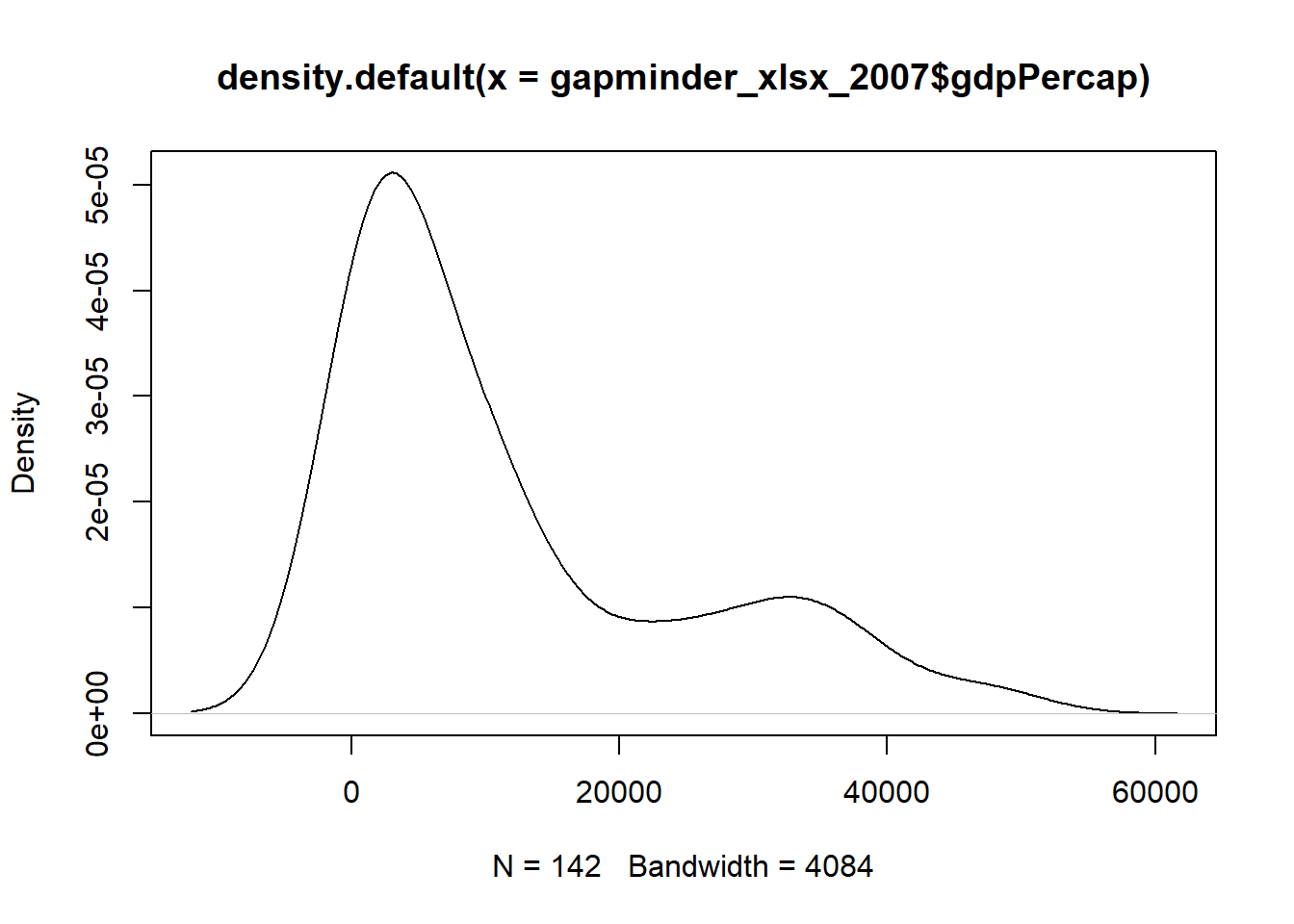
Outliers are identified using univariate plots such as histogram, density plot and boxplot.
# plotting variable using histogram
hist(gapminder_xlsx_2007$gdpPercap, breaks = 18)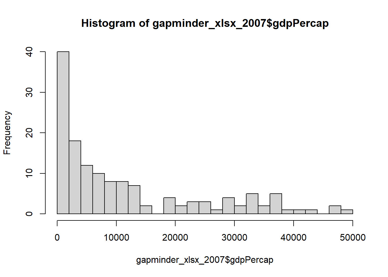
# boxplot of population
boxplot(gapminder_xlsx_2007$gdpPercap)
Of the above data visualizations, the boxplot is the most relevant as it shows both the spread of data and outliers. The boxplot reveals the following:
- minimum value,
- first quantile (Q1),
- median (second quantile),
- third quantile (Q3),
- maximum value excluding outliers and
- outliers.
The difference between Q3 and Q1 is known as the Interquartile Range (IQR). The outliers within the box plot are calculated as any value that falls beyond 1.5 * IQR.
The function boxplot.stats() computes the data that is used to draw the box plot. Using this function, we can get our outliers.
boxplot.stats(gapminder_xlsx_2007$gdpPercap)
#> $stats
#> [1]   277.5519  1598.4351  6124.3711 18008.9444 40675.9964
#>
#> $n
#> [1] 142
#>
#> $conf
#> [1] 3948.491 8300.251
#>
#> $out
#> [1] 47306.99 49357.19 47143.18 42951.65
The first element returned is the summary statistic as was calculated with summary().
boxplot.stats(gapminder_xlsx_2007$gdpPercap)$stats
#> [1]   277.5519  1598.4351  6124.3711 18008.9444 40675.9964
summary(gapminder_xlsx_2007$gdpPercap)
#>    Min. 1st Qu.  Median    Mean 3rd Qu.    Max.
#>   277.6  1624.8  6124.4 11680.1 18008.8 49357.2
The last element returned are the outliers.
boxplot.stats(gapminder_xlsx_2007$gdpPercap)$out
#> [1] 47306.99 49357.19 47143.18 42951.65
Recall outliers are calculated as 1.5 * IQR, this can be changed using the argument coef. By default, it is set to 1.5 but can be changed as need be.
# changing coef
boxplot.stats(gapminder_xlsx_2007$gdpPercap, coef = 0.8)$out
#>  [1] 34435.37 36126.49 33692.61 36319.24 35278.42 33207.08
#>  [7] 32170.37 39724.98 36180.79 40676.00 31656.07 47306.99
#> [13] 36797.93 49357.19 47143.18 33859.75 37506.42 33203.26
#> [19] 42951.65
boxplot.stats(gapminder_xlsx_2007$gdpPercap, coef = 1)$out
#>  [1] 34435.37 36126.49 36319.24 35278.42 39724.98 36180.79
#>  [7] 40676.00 47306.99 36797.93 49357.19 47143.18 37506.42
#> [13] 42951.65
boxplot.stats(gapminder_xlsx_2007$gdpPercap, coef = 1.2)$out
#> [1] 39724.98 40676.00 47306.99 49357.19 47143.18 42951.65

# selecting outliers
gapminder_xlsx_2007[gapminder_xlsx_2007$gdpPercap >= min(boxplot.stats(gapminder_xlsx_2007$gdpPercap)$out),]
#>            country continent year lifeExp       pop
#> 864         Kuwait      Asia 2007  77.588   2505559
#> 1152        Norway    Europe 2007  80.196   4627926
#> 1368     Singapore      Asia 2007  79.972   4553009
#> 1620 United States  Americas 2007  78.242 301139947
#>      gdpPercap      country_hun continent_hun
#> 864   47306.99           Kuvait         Ázsia
#> 1152  49357.19         Norvégia        Európa
#> 1368  47143.18        Szingapúr         Ázsia
#> 1620  42951.65 Egyesült Államok       Amerika
4.13 Dealing with duplicate values
4.13.1 Determining duplicate values
The function duplicated() determines which elements are duplicates in a vector or data frame while the function anyDuplicated() returns the index position of the first duplicate.
# checking for duplicates
duplicated(1:10)
#>  [1] FALSE FALSE FALSE FALSE FALSE FALSE FALSE FALSE FALSE
#> [10] FALSE

duplicated(c(2, 1, 3, 6, 2, 4, 7, 0, 3, 3, 2, 2, 8, 4, 0))
#>  [1] FALSE FALSE FALSE FALSE  TRUE FALSE FALSE FALSE  TRUE
#> [10]  TRUE  TRUE  TRUE FALSE  TRUE  TRUE

# get duplicate values
vt <- c(2, 1, 3, 6, 2, 4, 7, 0, 3, 3, 2, 2, 8, 4, 0)
vt[duplicated(c(2, 1, 3, 6, 2, 4, 7, 0, 3, 3, 2, 2, 8, 4, 0))]
#> [1] 2 3 3 2 2 4 0

# checking if an object contains any duplicates
any(duplicated(1:10))
#> [1] FALSE

any(duplicated(c(2, 1, 3, 6, 2, 4, 7, 0, 3, 3, 2, 2, 8, 4, 0)))
#> [1] TRUE

# get the first duplicate position
anyDuplicated(1:10)
#> [1] 0

anyDuplicated(c(2, 1, 3, 6, 2, 4, 7, 0, 3, 3, 2, 2, 8, 4, 0))
#> [1] 5
The function duplicated() and anyDuplicated() also work on data frames. The former drops unique rows while keeping duplicate rows.
movies_2006 <- mov[mov$Year == 2006, c(7,12)]
movies_2006 <- movies_2006[order(movies_2006$Year, movies_2006$Metascore),]
head(movies_2006)
#>     Year Metascore
#> 774 2006        36
#> 309 2006        45
#> 551 2006        45
#> 594 2006        45
#> 734 2006        46
#> 531 2006        47

# checking for any duplicates
any(duplicated(movies_2006))
#> [1] TRUE

anyDuplicated(movies_2006)
#> [1] 3

# checking for duplicates
duplicated(movies_2006)
#>  [1] FALSE FALSE  TRUE  TRUE FALSE FALSE FALSE FALSE FALSE
#> [10]  TRUE FALSE  TRUE FALSE FALSE  TRUE FALSE FALSE FALSE
#> [19]  TRUE  TRUE FALSE FALSE  TRUE  TRUE  TRUE FALSE  TRUE
#> [28] FALSE  TRUE FALSE FALSE FALSE FALSE  TRUE FALSE  TRUE
#> [37] FALSE FALSE  TRUE FALSE FALSE FALSE  TRUE  TRUE

# returning duplicates
movies_2006_dup <- movies_2006 [duplicated(movies_2006), ]
head(movies_2006_dup)
#>     Year Metascore
#> 551 2006        45
#> 594 2006        45
#> 859 2006        52
#> 960 2006        53
#> 902 2006        58
#> 670 2006        64
4.13.2 Get unique values
The function unique() extracts unique values from a vector or data frame.
# return unique values
unique(1:10)
#>  [1]  1  2  3  4  5  6  7  8  9 10

unique(c(2, 1, 3, 6, 2, 4, 7, 0, 3, 3, 2, 2, 8, 4, 0))
#> [1] 2 1 3 6 4 7 0 8

# return unique values using duplicated()
vt[!duplicated(c(2, 1, 3, 6, 2, 4, 7, 0, 3, 3, 2, 2, 8, 4, 0))]
#> [1] 2 1 3 6 4 7 0 8

# returning unique rows
movies_2006_uni <- unique(movies_2006)
head(movies_2006_uni)
#>     Year Metascore
#> 774 2006        36
#> 309 2006        45
#> 734 2006        46
#> 531 2006        47
#> 321 2006        48
#> 775 2006        51

# returning unique rows using duplicated()
movies_2006_uni <- subset(movies_2006, !duplicated(movies_2006))
head(movies_2006_uni)
#>     Year Metascore
#> 774 2006        36
#> 309 2006        45
#> 734 2006        46
#> 531 2006        47
#> 321 2006        48
#> 775 2006        51
4.14 Factors in Base R
4.14.1 What are factors?
Factors are variables in R which take on a limited number of different values which are usually known as categorical values e.g. male and female or months of the year. They can contain either strings or integers but are stored internally as a vector of integers with each integer corresponding to one category. Factors can either be ordered or unordered e.g. low, medium, high for ordered and male or female for unordered.
4.14.2 Creating a factor
While the function factor() is used to create a factor, the function is.factor() is used to check for factor.
# creating a factor
(fac <- factor(c('female', 'male', 'male', 'female', 'male', 'male', 'male', 'female')))
#> [1] female male   male   female male   male   male   female
#> Levels: female male

# looking at type and class
typeof(fac)
#> [1] "integer"
class(fac)
#> [1] "factor"

# checking if the object is a factor
is.factor(fac)
#> [1] TRUE
4.14.3 Factor attributes and structure
A factor has as attribute levels which represent the categories of the factor.
The function levels() is used to get and set levels while nlevels() returns the number of categories.
# get levels
levels(fac)
#> [1] "female" "male"

# set levels
(levels(fac) <- c('f', 'm'))
#> [1] "f" "m"

# resetting levels
(levels(fac) <- c('female', 'male'))
#> [1] "female" "male"

# number of categories
nlevels(fac)
#> [1] 2

# structure of the factor
str(fac)
#>  Factor w/ 2 levels "female","male": 1 2 2 1 2 2 2 1

attributes(fac)
#> $levels
#> [1] "female" "male"
#>
#> $class
#> [1] "factor"

# count of elements by category
table(fac)
#> fac
#> female   male
#>      3      5

# internally factors are stored as integers
unclass(fac)
#> [1] 1 2 2 1 2 2 2 1
#> attr(,"levels")
#> [1] "female" "male"
4.14.4 Rearranging levels
The argument levels is used to rearrange the levels of a factor.
lev <- c('male', 'female')
(fac1 <- factor(c('female', 'male', 'male', 'female', 'male', 'male', 'male', 'female'),
               levels = lev))
#> [1] female male   male   female male   male   male   female
#> Levels: male female

# comparing fac and fac1
attributes(fac)
#> $levels
#> [1] "female" "male"
#>
#> $class
#> [1] "factor"
attributes(fac1)
#> $levels
#> [1] "male"   "female"
#>
#> $class
#> [1] "factor"

table(fac)
#> fac
#> female   male
#>      3      5
table(fac1)
#> fac1
#>   male female
#>      5      3
4.14.5 Dropping levels
The function droplevels() is used to drop unused levels from a factor.
(fac1 <- factor(c('female', 'male', 'male', 'female', 'male', 'male', 'male', 'female'),
               levels = c('male', 'female', 'boy', 'girl')))
#> [1] female male   male   female male   male   male   female
#> Levels: male female boy girl
(fac1 <- droplevels(fac1))
#> [1] female male   male   female male   male   male   female
#> Levels: male female4.14.7 Ordered factors
Ordered factors are factors whose orders matter for example with grading; A is greater than B and B greater than C, and so forth. The argument order = TRUE is used to create an ordered factor. Also, the function ordered() can be used to create an ordered factor while the function is.ordered() is used to check for ordered factor. With ordered factors, we can use the function min() and max() on them to determine the minimum and maximum values, respectively.
(fac2 <- factor(c('female', 'male', 'male', 'female', 'male', 'male', 'male', 'female'),
               levels = lev,
               ordered = T))
#> [1] female male   male   female male   male   male   female
#> Levels: male < female
attributes(fac)
#> $levels
#> [1] "female" "male"
#>
#> $class
#> [1] "factor"
attributes(fac1)
#> $levels
#> [1] "M" "F"
#>
#> $class
#> [1] "factor"
attributes(fac2)
#> $levels
#> [1] "male"   "female"
#>
#> $class
#> [1] "ordered" "factor"

# getting minimum and maximum values
min(fac2)
#> [1] male
#> Levels: male < female
max(fac2)
#> [1] female
#> Levels: male < female

# checking for ordered factor
is.ordered(fac2)
#> [1] TRUE

ordered(c('female', 'male', 'male', 'female', 'male', 'male', 'male', 'female'))
#> [1] female male   male   female male   male   male   female
#> Levels: female < male
ordered(c('female', 'male', 'male', 'female', 'male', 'male', 'male', 'female'),
        levels = c('male', 'female'))
#> [1] female male   male   female male   male   male   female
#> Levels: male < female
The functions max() and min() do not work for fac and fac1 because they are not ordered, hence have no minimum or maximum.
4.14.8 Converting from character to factor
The function as.factor() converts to a factor, if possible but is less flexible than factor(). It is used when we do not care about levels, label or order.
month.name
#>  [1] "January"   "February"  "March"     "April"
#>  [5] "May"       "June"      "July"      "August"
#>  [9] "September" "October"   "November"  "December"
class(month.name)
#> [1] "character"

# converting to factor
(month_fac <- as.factor(month.name))
#>  [1] January   February  March     April     May
#>  [6] June      July      August    September October
#> [11] November  December
#> 12 Levels: April August December February January ... September
4.14.9 Converting from factor to character
The function as.character() converts from factor to character.
(month_char <- as.character(month_fac))
4.14.10 Converting from numeric to factor
The function cut() is used to convert from numeric vector to factor. It bins numbers into ranges which can be treated as categories.
scores <- c(15,65,68,46,15,61,32,13,15,46,13,21,89,89,44,51,32,16,18,95,46,16,65,46)

# create factors from numeric
cut(scores, breaks = 5)
#>  [1] (12.9,29.4] (62.2,78.6] (62.2,78.6] (45.8,62.2]
#>  [5] (12.9,29.4] (45.8,62.2] (29.4,45.8] (12.9,29.4]
#>  [9] (12.9,29.4] (45.8,62.2] (12.9,29.4] (12.9,29.4]
#> [13] (78.6,95.1] (78.6,95.1] (29.4,45.8] (45.8,62.2]
#> [17] (29.4,45.8] (12.9,29.4] (12.9,29.4] (78.6,95.1]
#> [21] (45.8,62.2] (12.9,29.4] (62.2,78.6] (45.8,62.2]
#> 5 Levels: (12.9,29.4] (29.4,45.8] ... (78.6,95.1]

# return categories
levels(cut(scores, breaks = 5))
#> [1] "(12.9,29.4]" "(29.4,45.8]" "(45.8,62.2]" "(62.2,78.6]"
#> [5] "(78.6,95.1]"

# number of levels
nlevels(cut(scores, breaks = 5))
#> [1] 5

# check class
class(cut(scores, breaks = 5))
#> [1] "factor"

# controlling breaks
cut(scores, breaks = c(0, 40 , 50, 60, 80, 100))
#>  [1] (0,40]   (60,80]  (60,80]  (40,50]  (0,40]   (60,80]
#>  [7] (0,40]   (0,40]   (0,40]   (40,50]  (0,40]   (0,40]
#> [13] (80,100] (80,100] (40,50]  (50,60]  (0,40]   (0,40]
#> [19] (0,40]   (80,100] (40,50]  (0,40]   (60,80]  (40,50]
#> Levels: (0,40] (40,50] (50,60] (60,80] (80,100]

# adding labels
cut(scores, breaks = c(0, 40 , 50, 60, 80, 100), labels = c('F', 'D', 'C', 'B', 'A'))
#>  [1] F B B D F B F F F D F F A A D C F F F A D F B D
#> Levels: F D C B A

# majority of the students failed
table(cut(scores, breaks = c(0, 40 , 50, 60, 80, 100), labels = c('F', 'D', 'C', 'B', 'A')))
#>
#>  F  D  C  B  A
#> 11  5  1  4  3
4.14.11 Converting from factor to numeric
To convert from a factor to numeric, the function as.numeric() does not work. To use it, we first have to convert the factor to character using as.character() or levels(fac)[fac]. Below we make use of both methods to achieve our objective.
num_vec <- c(15,65,68,46,15,61,32,13,15,46,13,21,89,89,44,51,32,16,18,95,46,16,65,46)
mean(num_vec)
#> [1] 42.375

#converting to factor
(fac3 <- factor(num_vec))
#>  [1] 15 65 68 46 15 61 32 13 15 46 13 21 89 89 44 51 32 16
#> [19] 18 95 46 16 65 46
#> Levels: 13 15 16 18 21 32 44 46 51 61 65 68 89 95

# calculating mean
mean(fac3)
#> [1] NA


# as.numeric() doesn't seem to work
mean(as.numeric(fac3))
#> [1] 6.958333


# using as.character
mean(as.numeric(as.character(fac3)))
#> [1] 42.375

# using levels()
mean(as.numeric(levels(fac3)[fac3]))
#> [1] 42.375
4.15 String manipulation with base R
4.15.1 String length and character count
The function length() returns the count of elements in a vector.
The function nchar() returns the count of letters in a string.
month.name
#>  [1] "January"   "February"  "March"     "April"
#>  [5] "May"       "June"      "July"      "August"
#>  [9] "September" "October"   "November"  "December"

#count of elements
length(month.name)
#> [1] 12

# count of letters
month.name
#>  [1] "January"   "February"  "March"     "April"
#>  [5] "May"       "June"      "July"      "August"
#>  [9] "September" "October"   "November"  "December"
nchar(month.name)
#>  [1] 7 8 5 5 3 4 4 6 9 7 8 8
4.15.2 Strings formatting (case-folding)
The functions toupper() and tolower() are used to convert to upper and lower cases, respectively while casefold() is a wrapper to these functions.
# uppercase
toupper(month.name)
#>  [1] "JANUARY"   "FEBRUARY"  "MARCH"     "APRIL"
#>  [5] "MAY"       "JUNE"      "JULY"      "AUGUST"
#>  [9] "SEPTEMBER" "OCTOBER"   "NOVEMBER"  "DECEMBER"
casefold(month.name, upper = TRUE)
#>  [1] "JANUARY"   "FEBRUARY"  "MARCH"     "APRIL"
#>  [5] "MAY"       "JUNE"      "JULY"      "AUGUST"
#>  [9] "SEPTEMBER" "OCTOBER"   "NOVEMBER"  "DECEMBER"

# lowercase
tolower(month.name)
#>  [1] "january"   "february"  "march"     "april"
#>  [5] "may"       "june"      "july"      "august"
#>  [9] "september" "october"   "november"  "december"
casefold(month.name, upper = FALSE)
#>  [1] "january"   "february"  "march"     "april"
#>  [5] "may"       "june"      "july"      "august"
#>  [9] "september" "october"   "november"  "december"
4.15.3 Join and Split strings
4.15.3.1 Joining strings using cat()
The function cat() converts its arguments to strings and concatenates them after appending a separator string (given by sep) to them.
a <- month.name[1]
b <- month.name[2]
c <- month.name[3]
cat(b,'comes after', a ,'but comes before', c)
#> February comes after January but comes before March
cat(b,'comes before', a ,'but comes after', c, sep = '/')
#> February/comes before/January/but comes after/March
cat(month.name[1:6], sep = ' - ')
#> January - February - March - April - May - June
cat(month.name[1:6], sep = ' <> ')
#> January <> February <> March <> April <> May <> June
Newlines and tabs can be added by using \n for newline and \t for tabs.
# adding a new line
cat(b,'comes after\n', a ,'but comes before', c)
#> February comes after
#>  January but comes before March

# adding a tab
cat(b,'comes after\t', a ,'but comes before', c)
#> February comes after  January but comes before March
The function cat() can write its output directly to a file if a file name is passed to it.
# writing to disc
cat(month.name, sep = ' <> ', file = "output/data/months.txt")

# checking if file exists
file.exists('output/data/months.txt')
#> [1] TRUE

# removing file
file.remove('output/data/months.txt')
#> [1] TRUE
4.15.3.2 Joining strings using paste() and paste0()
The function paste() concatenate vectors after converting them to character and separating them by a string given by sep. It concatenates multiple vectors element by element to give a new character vector and if one is shorter, recycling occurs with zero-length arguments being recycled to ““.
With a single vector, it is simply converted to a character vector and if the argument collapse is set, the elements are condensed into a single string.
The function paste0(...) is equivalent to paste(…, sep = ’’), but slightly more efficient.
# combining elements into a character vector
paste('a', 'b')
#> [1] "a b"
paste(1, 2, 3, 4)
#> [1] "1 2 3 4"


# using a sep
paste('a', 'b', sep = '')
#> [1] "ab"
paste(1, 2, 3, 4, sep = '')
#> [1] "1234"


# using paste0
paste0('a', 'b')
#> [1] "ab"
paste0(1, 2, 3 ,4)
#> [1] "1234"

# on a single vector
paste(c('a', 'b'), sep = ' <> ')
#> [1] "a" "b"
paste(c(1, 2), sep = ' <> ')
#> [1] "1" "2"

# two or more vectors
paste(c('a', 'b'), c('c', 'd'), sep = ' <> ')
#> [1] "a <> c" "b <> d"
paste0(c('a', 'b'), c('c', 'd'))
#> [1] "ac" "bd"
paste0(1:5, 6:10)
#> [1] "16"  "27"  "38"  "49"  "510"
paste(1:5, 10:20)
#>  [1] "1 10" "2 11" "3 12" "4 13" "5 14" "1 15" "2 16" "3 17"
#>  [9] "4 18" "5 19" "1 20"
paste(1:5, 10:20, c('a','b','c'))
#>  [1] "1 10 a" "2 11 b" "3 12 c" "4 13 a" "5 14 b" "1 15 c"
#>  [7] "2 16 a" "3 17 b" "4 18 c" "5 19 a" "1 20 b"

# combining character and variables with paste
paste(b,'comes after', a ,'but comes before', c)
#> [1] "February comes after January but comes before March"
paste(b,'comes after', a ,'but comes before', c, sep = "    ")
#> [1] "February    comes after    January    but comes before    March"
paste(b,'comes after', a ,'but comes before', c, sep = "/")
#> [1] "February/comes after/January/but comes before/March"
paste('version 1.', 1:5, sep = '')
#> [1] "version 1.1" "version 1.2" "version 1.3" "version 1.4"
#> [5] "version 1.5"

# combining character and variables with paste0
paste0(b,' comes after ', a ,' but comes before ', c)
#> [1] "February comes after January but comes before March"
paste0(b,'    comes after    ', a ,'    but comes before    ', c)
#> [1] "February    comes after    January    but comes before    March"

paste0(b,'/comes after/', a ,'/but comes before/', c)
#> [1] "February/comes after/January/but comes before/March"
paste0('version 1.', 1:5)
#> [1] "version 1.1" "version 1.2" "version 1.3" "version 1.4"
#> [5] "version 1.5"
The collapse argument is used to collapse elements returned into a single string.
# collapsing vectors
paste(1:10, collapse = '~')
#> [1] "1~2~3~4~5~6~7~8~9~10"
paste(c('a', 'b'), c('c', 'd'), collapse = ' <> ')
#> [1] "a c <> b d"
paste0(c('a', 'b'), c('c', 'd'), collapse = ' <> ')
#> [1] "ac <> bd"

paste0(1:5, 6:10, collapse = '--')
#> [1] "16--27--38--49--510"
paste(month.name[1:6], collapse = " - ")
#> [1] "January - February - March - April - May - June"
4.15.3.3 Joining strings using sprintf()
The function sprintf() returns a character vector containing a formatted combination of text and variable values.
The format of the variables is passed using one of the following characters aAdifeEgGosxX% and should start with %.
4.15.3.3.1 Formatting with integers
The command %d is used for formatting integers.
# using an integer as a variable
x <- 2
sprintf('%d * %d = %d', x, x, x ** 2)
#> [1] "2 * 2 = 4"
x <- c(1:4)
y <- x ** 2
sprintf('%d squared is equal to %d', x, y)
#> [1] "1 squared is equal to 1"  "2 squared is equal to 4"
#> [3] "3 squared is equal to 9"  "4 squared is equal to 16"

### padding integers with zeros
num <- c(123, 1, 100, 200, 10200, 25000)
sprintf('my registration number is %05d', num)
#> [1] "my registration number is 00123"
#> [2] "my registration number is 00001"
#> [3] "my registration number is 00100"
#> [4] "my registration number is 00200"
#> [5] "my registration number is 10200"
#> [6] "my registration number is 25000"
4.15.3.3.2 Formatting with strings
The command %s is used for formatting strings.
# using a string as a variable
x <- 'my name is'
y <- 'james'
z <- 'london'
sprintf('%s %s and i live and work in %s', x, y, z)
#> [1] "my name is james and i live and work in london"

# combining strings and integers
x <- 'my name is'
y <- 'james'
z <- 35
sprintf('%s %s and i am %d years', x, y, z)
#> [1] "my name is james and i am 35 years"

names = c('paul', 'alphonse', 'michael', 'james', 'samson', 'terence', 'derin')
age = c(30, 35, 32, 37, 29, 40, 30)
sprintf('i am %s and i am %d years old', names, age)
#> [1] "i am paul and i am 30 years old"
#> [2] "i am alphonse and i am 35 years old"
#> [3] "i am michael and i am 32 years old"
#> [4] "i am james and i am 37 years old"
#> [5] "i am samson and i am 29 years old"
#> [6] "i am terence and i am 40 years old"
#> [7] "i am derin and i am 30 years old"
4.15.3.3.3 Formatting with doubles or floating-points
The command %f is used for formatting doubles while either %e or %E for formatting exponential.
# using doubles as a variable
x <- 1000/6
sprintf('1000 divided by 3 is %f', x)
#> [1] "1000 divided by 3 is 166.666667"

# rounding a double to the nearest decimal
sprintf('1000 divided by 3 is %.3f', x)
#> [1] "1000 divided by 3 is 166.667"
sprintf('1000 divided by 3 is %.2f', x)
#> [1] "1000 divided by 3 is 166.67"
sprintf('1000 divided by 3 is %.1f', x)
#> [1] "1000 divided by 3 is 166.7"

# rounding a double to the nearest whole number
sprintf('1000 divided by 3 is %1.f', x)
#> [1] "1000 divided by 3 is 167"

# printing a plus (+) in front of a double
sprintf('+1000 divided by 3 is %+.1f', x)
#> [1] "+1000 divided by 3 is +166.7"

# printing space in front of a double
sprintf('1000 divided by 3 is %f', x)
#> [1] "1000 divided by 3 is 166.666667"
sprintf('1000 divided by 3 is % f', x)
#> [1] "1000 divided by 3 is  166.666667"

# exponential
sprintf("%e", pi)
#> [1] "3.141593e+00"
4.15.3.4 Splitting strings using strsplit()
The function strsplit() splits the elements of a character vector into substrings by a specific split character. It returns a list.
str(strsplit(c('2020-01-01', '2019-03-31', '2018-06-30'), split = "-"))
#> List of 3
#>  $ : chr [1:3] "2020" "01" "01"
#>  $ : chr [1:3] "2019" "03" "31"
#>  $ : chr [1:3] "2018" "06" "30"
str(strsplit(c('2020 01 01', '2019 03 31', '2018 06 30'), split = " "))
#> List of 3
#>  $ : chr [1:3] "2020" "01" "01"
#>  $ : chr [1:3] "2019" "03" "31"
#>  $ : chr [1:3] "2018" "06" "30"
str(strsplit(c('2020, 01, 01', '2019, 03, 31', '2018, 06, 30'), split = ", "))
#> List of 3
#>  $ : chr [1:3] "2020" "01" "01"
#>  $ : chr [1:3] "2019" "03" "31"
#>  $ : chr [1:3] "2018" "06" "30"
4.15.4 Extract and Replace part of strings
4.15.4.1 Extracting substring using substr()
The function substr() extracts a substring from a string by indexing. It uses start for the beginning position and stop for the ending position. It is like indexing but applied to a string.
4.15.4.2 Replacing substring using substr()
The function substr() is also used to replace substring in a string by assigning a different string to the extracted substring.
var <- c('2020-01-01', '2019-03-31', '2018-06-30')
substr(var, start = 1, stop = 4) <- c('2010', '2011', '2012')
var
#> [1] "2010-01-01" "2011-03-31" "2012-06-30"

weekdays <- c('monday', 'tuesday', 'wednesday', 'thursday', 'friday', 'saturday', 'sunday')
substr(weekdays, start = 1, stop = 1) <- toupper(substr(weekdays, start = 1, stop = 1))
weekdays
#> [1] "Monday"    "Tuesday"   "Wednesday" "Thursday"
#> [5] "Friday"    "Saturday"  "Sunday"
4.15.4.3 Replacing substrings using sub()
The function sub() replaces a substring at first occurrence in a string.
4.15.4.4 Replacing substrings using gsub()
The function gsub() replaces a substring throughout a string.
4.15.4.5 Replacing substring using chartr()
The function chartr() replaces a substring throughout a string.
4.15.5 Pattern matching using regular expression
4.15.5.1 Regex functions
4.15.5.1.1 The grep() function
The function grep() returns the index position or value of elements that match a pattern.
# returning index position
month.name
#>  [1] "January"   "February"  "March"     "April"
#>  [5] "May"       "June"      "July"      "August"
#>  [9] "September" "October"   "November"  "December"
grep(pattern = 'uary', month.name)
#> [1] 1 2

# returning values
grep('uary', month.name, value = TRUE)
#> [1] "January"  "February"

# ignoring case
grep('ju', month.name, value = TRUE)
#> character(0)
grep('ju', month.name, ignore.case = TRUE, value = TRUE)
#> [1] "June" "July"
4.15.5.2 The grepl() function
The function grepl() returns TRUE for pattern match and FALSE for no pattern match.
4.15.5.3 The regexpr() function
The function regexpr() returns the position of the first pattern match in an element with -1 representing no pattern match.
regexpr('ber', month.name, ignore.case = TRUE)
#>  [1] -1 -1 -1 -1 -1 -1 -1 -1  7  5  6  6
#> attr(,"match.length")
#>  [1] -1 -1 -1 -1 -1 -1 -1 -1  3  3  3  3
#> attr(,"index.type")
#> [1] "chars"
#> attr(,"useBytes")
#> [1] TRUE
(st <- state.name[20:25])
#> [1] "Maryland"      "Massachusetts" "Michigan"
#> [4] "Minnesota"     "Mississippi"   "Missouri"
regexpr('ss', st, ignore.case = TRUE)
#> [1] -1  3 -1 -1  3  3
#> attr(,"match.length")
#> [1] -1  2 -1 -1  2  2
#> attr(,"index.type")
#> [1] "chars"
#> attr(,"useBytes")
#> [1] TRUE
4.15.5.4 The gregexpr() function
The function gregexpr() returns the position of all pattern matches in an element with -1 representing no pattern match.
# same as as.list(regexpr())
(st <- state.name[23:25])
#> [1] "Minnesota"   "Mississippi" "Missouri"
gregexpr('ss', st, ignore.case = TRUE)
#> [[1]]
#> [1] -1
#> attr(,"match.length")
#> [1] -1
#> attr(,"index.type")
#> [1] "chars"
#> attr(,"useBytes")
#> [1] TRUE
#>
#> [[2]]
#> [1] 3 6
#> attr(,"match.length")
#> [1] 2 2
#> attr(,"index.type")
#> [1] "chars"
#> attr(,"useBytes")
#> [1] TRUE
#>
#> [[3]]
#> [1] 3
#> attr(,"match.length")
#> [1] 2
#> attr(,"index.type")
#> [1] "chars"
#> attr(,"useBytes")
#> [1] TRUE
4.15.5.5 Regex Operations
4.15.5.5.1 Matching spaces
- [[:blank:]] matches space and tab characters
- [[:space:]] matches tab, newline, vertical tab, form feed, carriage return, and space
- \s matches space character
- \S matches non-space character
# creating a character vector
var <- c('2020 01 01', '2019 03 31', '2018 06 30')

# POSIX Character
gsub('[[:space:]]', '-', var)
#> [1] "2020-01-01" "2019-03-31" "2018-06-30"
gsub('[[:space:]]', '/', var)
#> [1] "2020/01/01" "2019/03/31" "2018/06/30"
gsub('[[:blank:]]', '_', var)
#> [1] "2020_01_01" "2019_03_31" "2018_06_30"
gsub('[[:blank:]]', '/', var)
#> [1] "2020/01/01" "2019/03/31" "2018/06/30"

# Sequences
gsub('\\s', '-', var)
#> [1] "2020-01-01" "2019-03-31" "2018-06-30"
gsub('\\s', '/', var)
#> [1] "2020/01/01" "2019/03/31" "2018/06/30"
gsub('\\s', '_', var)
#> [1] "2020_01_01" "2019_03_31" "2018_06_30"
gsub('\\s', '/', var)
#> [1] "2020/01/01" "2019/03/31" "2018/06/30"

# using strsplit() to split based on a pattern
var <- c('2020 01 01', '2019 03 31', '2018 06 30')
str(strsplit(var, split = '\\s'))
#> List of 3
#>  $ : chr [1:3] "2020" "01" "01"
#>  $ : chr [1:3] "2019" "03" "31"
#>  $ : chr [1:3] "2018" "06" "30"

# matching non-space character with \\S
var <- c('2020 01 01', '2019 03 31', '2018 06 30')
gsub('\\S', '-', var)
#> [1] "---- -- --" "---- -- --" "---- -- --"
gsub('\\S', '/', var)
#> [1] "//// // //" "//// // //" "//// // //"
gsub('\\S', '_', var)
#> [1] "____ __ __" "____ __ __" "____ __ __"
gsub('\\S', '/', var)
#> [1] "//// // //" "//// // //" "//// // //"
Matching alphabetic characters
- [[:alpha:]] matches alphabetic characters
- [[:lower:]] matches lowercase characters
- [[:upper:]] matches uppercase characters
var <- 'a1b2c3d4e5f'

# matching alphabetic characters
gsub('[[:alpha:]]', '', var)
#> [1] "12345"
gsub('[[:alpha:]]', '-', var)
#> [1] "-1-2-3-4-5-"

# matching lowercase letters
gsub('[[:lower:]]', '', month.name)
#>  [1] "J" "F" "M" "A" "M" "J" "J" "A" "S" "O" "N" "D"

# matching uppercase letters
gsub('[[:upper:]]', '', month.name)
#>  [1] "anuary"   "ebruary"  "arch"     "pril"     "ay"
#>  [6] "une"      "uly"      "ugust"    "eptember" "ctober"
#> [11] "ovember"  "ecember"
Matching numerical digits
- [[:digit:]] and \d matches numbers from 0-9.
var <- 'a1b2c3d4e5f'

# POSIX Character
gsub('[[:digit:]]', '', var)
#> [1] "abcdef"
gsub('[[:digit:]]', '-', var)
#> [1] "a-b-c-d-e-f"

# Sequences
gsub('\\d', '', var)
#> [1] "abcdef"
gsub('\\d', '-', var)
#> [1] "a-b-c-d-e-f"
Matching letters and numbers (alphanumeric characters)
- [[:alnum:]] matches alphanumeric characters ([[:alpha:]] and [[:digit:]])
- [[:xdigit:]] matches Hexadecimal digits (0 1 2 3 4 5 6 7 8 9 A B C D E F a b c d e f)
- \w matches word characters
var <- 'a1@; 2#4c $8`*%f^!1~0&^h*()j'

# alphanumeric characters
gsub('[[:alnum:]]', '', var)
#> [1] "@; # $`*%^!~&^*()"
gsub('[[:alnum:]]', '-', var)
#> [1] "--@; -#-- $-`*%-^!-~-&^-*()-"

# Hexadecimal digits
gsub('[[:xdigit:]]', '', var)
#> [1] "@; # $`*%^!~&^h*()j"
gsub('[[:xdigit:]]', '-', var)
#> [1] "--@; -#-- $-`*%-^!-~-&^h*()j"

# matching word characters
gsub('\\w', '', var)
#> [1] "@; # $`*%^!~&^*()"
gsub('\\w', '-', var)
#> [1] "--@; -#-- $-`*%-^!-~-&^-*()-"
Matching punctuation
- [[:punct:]] matches punctuation characters.
- \W matches non-word characters.
var <- 'a1@; 2#4c $8`*%f^!1~0&^h*()j'

# matching punctuation characters
gsub('[[:punct:]]', '', var)
#> [1] "a1 24c 8f10hj"
gsub('[[:punct:]]', '-', var)
#> [1] "a1-- 2-4c -8---f--1-0--h---j"

# matching non-word characters
gsub('\\W', '', var)
#> [1] "a124c8f10hj"
gsub('\\W', '-', var)
#> [1] "a1---2-4c--8---f--1-0--h---j"
Matching letters, numbers, and punctuation
- [[:graph:]] matches graphical characters ([[:alpha:]] and [[:punct:]])
- . matches any character (except newline character)
# matching graphical characters
var <- 'a1@; 2#4c $8%f^!10&^h*()j'
gsub('[[:graph:]]', ' ', var)
#> [1] "                         "

# matching anything but newline characters
var <- 'a1@; 2#4c $8%f^!10&^h*()j'
gsub('.', ' ', var)
#> [1] "                         "
Matching whitespace
- \s is used to match whitespaces.
# removing whitespace
gsub('\\s', '', c(' 2020-01-01 ', ' 2019-03-31 ', ' 2018-06-30 '))
#> [1] "2020-01-01" "2019-03-31" "2018-06-30"
Matching a newline
- \n is used to match a newline.
cat('good morning \n i am fru kinglsy \n i will be your instructor')
#> good morning
#>  i am fru kinglsy
#>  i will be your instructor

# replacing newline with tab
gsub('\\n', '\t', 'good morning \n i am fru kinglsy \n i will be your instructor')
#> [1] "good morning \t i am fru kinglsy \t i will be your instructor"

# print it out
cat(gsub('\\n', '\t', 'good morning \n i am fru kinglsy \n i will be your instructor'))
#> good morning      i am fru kinglsy    i will be your instructor
Matching tab
- \t is used to match tabs.
# replacing tab by newline
gsub('\\t', '\n', 'good morning \t i am fru kinglsy \t i will your instructor')
#> [1] "good morning \n i am fru kinglsy \n i will your instructor"

# printing it out
cat(gsub('\\t', '\n', 'good morning \t i am fru kinglsy \t i will your instructor'))
#> good morning
#>  i am fru kinglsy
#>  i will your instructor
4.15.5.6 Matching metacharacters
Metacharacters consist of non-alphanumeric symbols such as $ . ^ * | + ! ? () {} []. They are matched, by escaping them with a double backslash \.
# matching $
sales <-
  c('$25000', '$20000', '$22500', '$24000', '$30000', '$35000')
sub('\\$', '', sales)
#> [1] "25000" "20000" "22500" "24000" "30000" "35000"

# matching +
sales <-
  c('+25000', '+20000', '+22500', '+24000', '+30000', '+35000')
sub('\\+', '', sales)
#> [1] "25000" "20000" "22500" "24000" "30000" "35000"

# matching .
dates <-
  c('01.01.2012', '01.02.2012', '01.03.2012', '01.04.2012', '01.05.2012', '01.06.2012')
gsub('\\.', '-', dates)
#> [1] "01-01-2012" "01-02-2012" "01-03-2012" "01-04-2012"
#> [5] "01-05-2012" "01-06-2012"

# matching *
dates <-
  c('01*01*2012', '01*02*2012', '01*03*2012', '01*04*2012', '01*05*2012', '01*06*2012')
gsub('\\*', '-', dates)
#> [1] "01-01-2012" "01-02-2012" "01-03-2012" "01-04-2012"
#> [5] "01-05-2012" "01-06-2012"
#> [1] "01-01-2012" "01-02-2012" "01-03-2012" "01-04-2012" "01-05-2012"
#> [6] "01-06-2012"

# matching ^
dates <-
  c('01^01^2012', '01^02^2012', '01^03^2012', '01^04^2012', '01^05^2012', '01^06^2012')
gsub('\\^', '-', dates)
#> [1] "01-01-2012" "01-02-2012" "01-03-2012" "01-04-2012"
#> [5] "01-05-2012" "01-06-2012"

# matching |
dates <-
  c('01|01|2012', '01|02|2012', '01|03|2012', '01|04|2012', '01|05|2012', '01|06|2012')
gsub('\\|', '-', dates)
#> [1] "01-01-2012" "01-02-2012" "01-03-2012" "01-04-2012"
#> [5] "01-05-2012" "01-06-2012"

# matching \
dates <-
  c('01\\01\\2012', '01\\02\\2012', '01\\03\\2012',
    '01\\04\\2012', '01\\05\\2012', '01\\06\\2012')
gsub('\\\\', '-', dates)
#> [1] "01-01-2012" "01-02-2012" "01-03-2012" "01-04-2012"
#> [5] "01-05-2012" "01-06-2012"

# matching \\.
dates <-
  c('01\\.01\\.2012', '01\\.02\\.2012', '01\\.03\\.2012',
    '01\\.04\\.2012', '01\\.05\\.2012', '01\\.06\\.2012')
gsub('\\\\\\.', '-', dates)
#> [1] "01-01-2012" "01-02-2012" "01-03-2012" "01-04-2012"
#> [5] "01-05-2012" "01-06-2012"
Alternates and ranges
Either or (|)
# replacing either uary or ember or ober
gsub('uary|ember|ober', '-', month.name)
#>  [1] "Jan-"   "Febr-"  "March"  "April"  "May"    "June"
#>  [7] "July"   "August" "Sept-"  "Oct-"   "Nov-"   "Dec-"
set of characters ([]) matches a set of characters.
ranges (-) matches a range of characters.
# matching vowels
gsub('[aeiou]', '*', month.name)
#>  [1] "J*n**ry"   "F*br**ry"  "M*rch"     "Apr*l"
#>  [5] "M*y"       "J*n*"      "J*ly"      "A*g*st"
#>  [9] "S*pt*mb*r" "Oct*b*r"   "N*v*mb*r"  "D*c*mb*r"

# matching lower cases
gsub('[a-z]', '*', month.name)
#>  [1] "J******"   "F*******"  "M****"     "A****"
#>  [5] "M**"       "J***"      "J***"      "A*****"
#>  [9] "S********" "O******"   "N*******"  "D*******"

# matching upper cases
gsub('[A-Z]', '*', month.name)
#>  [1] "*anuary"   "*ebruary"  "*arch"     "*pril"
#>  [5] "*ay"       "*une"      "*uly"      "*ugust"
#>  [9] "*eptember" "*ctober"   "*ovember"  "*ecember"

# matching the letters m to z
gsub('[m-z]', '*', month.name)
#>  [1] "Ja**a**"   "Feb**a**"  "Ma*ch"     "A**il"
#>  [5] "Ma*"       "J**e"      "J*l*"      "A*g***"
#>  [9] "Se**e*be*" "Oc**be*"   "N**e*be*"  "Dece*be*"

# matching the numbers 0 to 9
gsub('[0-9]', '*', c('1a8g9u93l48p51359p78'))
#> [1] "*a*g*u**l**p*****p**"

# matching the numbers 1 to 5
gsub('[1-5]', '*', c('1a8g9u93l48p51359p78'))
#> [1] "*a8g9u9*l*8p****9p78"

# matching alphanumeric
gsub('[a-zA-Z0-9]', '*', c('1a8#g9u/93l48p51*395(9p78'))
#> [1] "***#***/************(****"
Not [^abc]
# matching everything but vowels
gsub('[^aeiou]', '*', month.name)
#>  [1] "*a*ua**"   "*e**ua**"  "*a***"     "***i*"
#>  [5] "*a*"       "*u*e"      "*u**"      "*u*u**"
#>  [9] "*e**e**e*" "***o*e*"   "*o*e**e*"  "*e*e**e*"

# matching everything but lowercase letters
gsub('[^a-z]', '*', month.name)
#>  [1] "*anuary"   "*ebruary"  "*arch"     "*pril"
#>  [5] "*ay"       "*une"      "*uly"      "*ugust"
#>  [9] "*eptember" "*ctober"   "*ovember"  "*ecember"
Anchors
- ^ matches a pattern at the start of a string. / $ matches a pattern at the end of a string.
# start of a string
gsub('^J', 'j', month.name)
#>  [1] "january"   "February"  "March"     "April"
#>  [5] "May"       "june"      "july"      "August"
#>  [9] "September" "October"   "November"  "December"

# end of a string
gsub('ber$', 'ba', month.name)
#>  [1] "January"  "February" "March"    "April"    "May"
#>  [6] "June"     "July"     "August"   "Septemba" "Octoba"
#> [11] "Novemba"  "Decemba"
Quantifiers
- matches a pattern 0 or more times
- matches a pattern 1 or more times
- ? matches a pattern 0 or one time
- x{m} matches x exactly m times
- x{m,} matches x exactly m or more times
- x{m,n} matches x exactly m or n times
# match 's' zero or one time
grep('s?', month.name, value = TRUE)
#>  [1] "January"   "February"  "March"     "April"
#>  [5] "May"       "June"      "July"      "August"
#>  [9] "September" "October"   "November"  "December"

# match 'J' one or more times
grep('J+', month.name, value = TRUE)
#> [1] "January" "June"    "July"

# match 'e' one or more times
grep('e+', state.name, value = TRUE)
#>  [1] "Connecticut"   "Delaware"      "Georgia"
#>  [4] "Kentucky"      "Maine"         "Massachusetts"
#>  [7] "Minnesota"     "Nebraska"      "Nevada"
#> [10] "New Hampshire" "New Jersey"    "New Mexico"
#> [13] "New York"      "Oregon"        "Pennsylvania"
#> [16] "Rhode Island"  "Tennessee"     "Texas"
#> [19] "Vermont"       "West Virginia"

# matched 'y', zero or more times
grep('y*', month.name, value = TRUE)
#>  [1] "January"   "February"  "March"     "April"
#>  [5] "May"       "June"      "July"      "August"
#>  [9] "September" "October"   "November"  "December"

# matched 'a', zero or more times
grep('a*', month.name, value = TRUE)
#>  [1] "January"   "February"  "March"     "April"
#>  [5] "May"       "June"      "July"      "August"
#>  [9] "September" "October"   "November"  "December"

# match 'a' zero or more times and 'y'
grep('a*y', month.name, value = TRUE)
#> [1] "January"  "February" "May"      "July"

# match 'y' zero or more times and 'a'
grep('y*a', month.name, value = TRUE)
#> [1] "January"  "February" "March"    "May"

# match 's', exactly 2 times
grep(pattern = "s{2}", state.name, value = TRUE)
#> [1] "Massachusetts" "Mississippi"   "Missouri"
#> [4] "Tennessee"

# match 's', exactly 1 or more times
grep(pattern = "s{1,}", state.name, value = TRUE)
#>  [1] "Alaska"        "Arkansas"      "Illinois"
#>  [4] "Kansas"        "Louisiana"     "Massachusetts"
#>  [7] "Minnesota"     "Mississippi"   "Missouri"
#> [10] "Nebraska"      "New Hampshire" "New Jersey"
#> [13] "Pennsylvania"  "Rhode Island"  "Tennessee"
#> [16] "Texas"         "Washington"    "West Virginia"
#> [19] "Wisconsin"

# match 's', exactly 1 or 2 times
grep(pattern = "s{1,2}", state.name, value = TRUE)
#>  [1] "Alaska"        "Arkansas"      "Illinois"
#>  [4] "Kansas"        "Louisiana"     "Massachusetts"
#>  [7] "Minnesota"     "Mississippi"   "Missouri"
#> [10] "Nebraska"      "New Hampshire" "New Jersey"
#> [13] "Pennsylvania"  "Rhode Island"  "Tennessee"
#> [16] "Texas"         "Washington"    "West Virginia"
#> [19] "Wisconsin"
Groups
() matches group patterns.
# match 2 repeating 's' followed by an 'e'
grep(pattern = '(s{2})e', state.name, value = TRUE)
#> [1] "Tennessee"