9 Summary

9.1 RMarkdown

With R markdown, it is easy to reproduce not only the analysis used, but also the entire report. The advantage of using R markdown (versus a script) is that you can combine computation with explanation. In other words, you can weave the outputs of your R code, like figures and tables, with text to create a report.

	RMarkdown	R script
File extension	.Rmd	.R
File contents	R code + Markdown text + YAML header	R code
Reproducibility	analysis + entire report	only the analysis
Output format	PDF, HTML, Word DOCX	-

9.2 Advanced data manipulation

	Base R	Tidyverse R
Most used function	[]	%>%
Import	read.table() rio::import() Link	readr::read_delim() Link
Export	write.table() rio::export() Link	readr::write_delim() Link
Inspecting dataset	str() Link	dplyr::glimpse() Link
Working with factors	factor() Link	forcats::fct_infreq() Link
Working with strings	paste() Link	stringr::str_c() Link
Working with column names	names() Link	dplyr::rename() Link
Working with row names	rownames() Link	tibble::rowid_to_column() Link
Filtering columns	[] Link	dplyr::select() Link
Filtering rows	[] Link	dplyr::filter() Link
Sorting rows	[] Link	dplyr::arrange() Link
Changing your data	cut() Link	dplyr::mutate() Link
Summarising data	aggregate() Link	dplyr::summarise() Link
Combining datasets	merge() Link	dplyr::left_join() Link
Reshaping data	reshape2::melt() reshape2::dcast() Link	tidyr::pivot_longer() tidyr::pivot_wider() Link

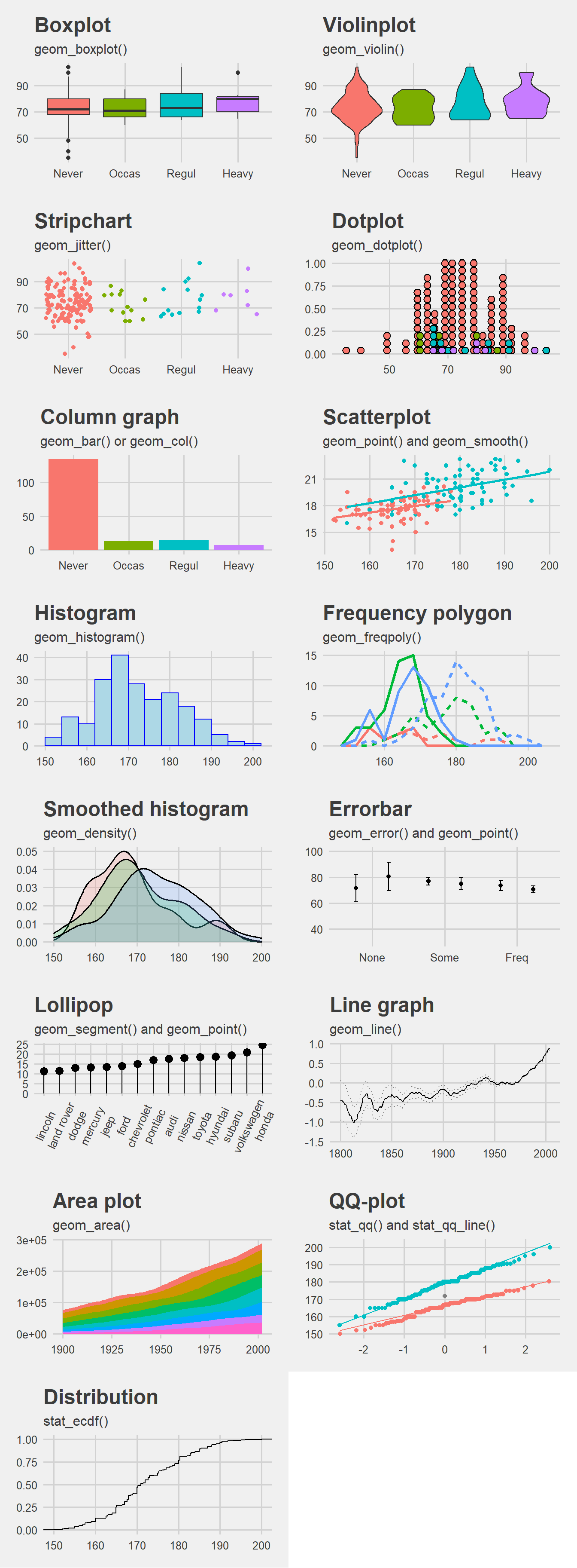
9.3 Modern graphics in R - ggplot2

9.3.1 The grammar of graphics

The grammar of graphics lies at the heart of ggplot2 and also lies at the heart of how we define our data visualizations.⁵

Table 9.1: The Grammar of Graphics

Component	Description
Data	Raw data that we’d like to visualize
Geometries	Shapes that we use to visualize
Aesthetics	Properties of geometries (size, color etc.)
Mapping	Mapping between data and aesthetics

library(tidyverse)
# a tibble for data, 3 rows, 4 columns
d.tbl <- tribble(
  ~group, ~score.1, ~score.2, ~score.3,
  "AA", 15, 42, 12, 
  "BB", 20, 28, 18,
  "CC", 35, 12, 21
)

# Scatterplot
#   Data: d.tbl
#   Geometry: point
#   Aesthetics: x, y
#   Mapping: x=score.1, y=score.2
ggplot(data=d.tbl, mapping=aes(x=score.1, y=score.2)) + geom_point()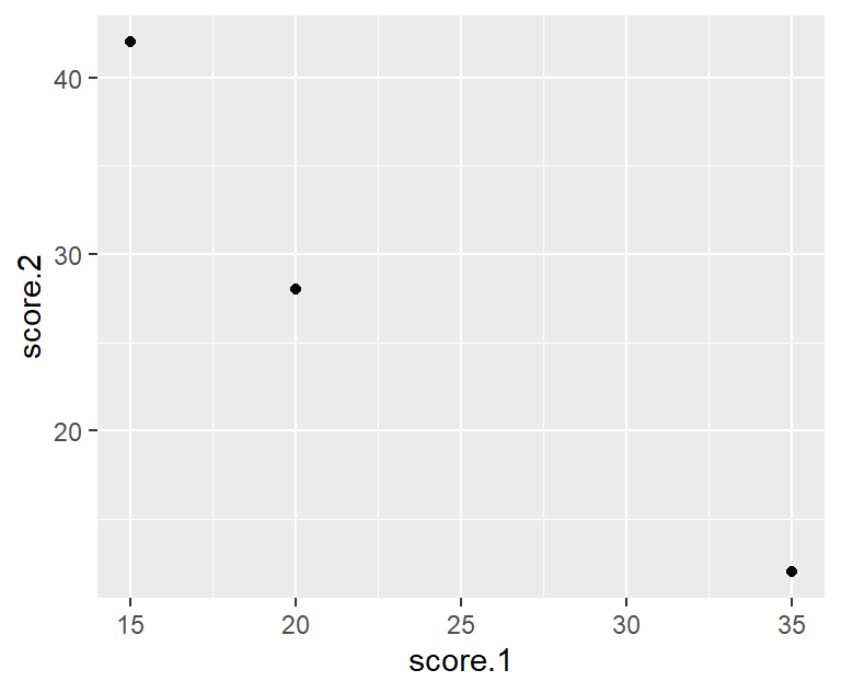

# Column Graph
#   Data: d.tbl
#   Geometry: column
#   Aesthetics: x, y
#   Mapping: x=score.1, y=score.2
ggplot(data=d.tbl, mapping=aes(x=score.1, y=score.2)) + geom_col()

# Line Graph
#   Data: d.tbl
#   Geometry: line
#   Aesthetics: x, y
#   Mapping: x=score.1, y=score.2
ggplot(data=d.tbl, mapping=aes(x=score.1, y=score.2)) + geom_line()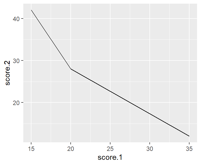

# all in one
ggplot(data=d.tbl, mapping=aes(x=score.1, y=score.2)) + 
  geom_point() + geom_col() + geom_line()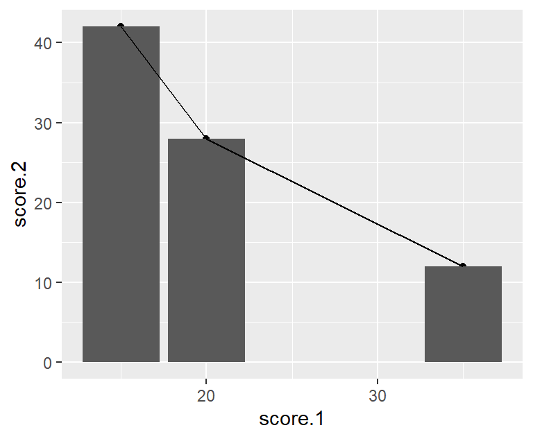

# Scatterplot
#   Data: d.tbl
#   Geometry: point
#   Aesthetics: x, y, size, color
#   Mapping: x=score.1, y=score.2, size=score.3, color=group
ggplot(data=d.tbl, 
       mapping=aes(x=score.1, y=score.2, size=score.3, color=group)) + 
  geom_point()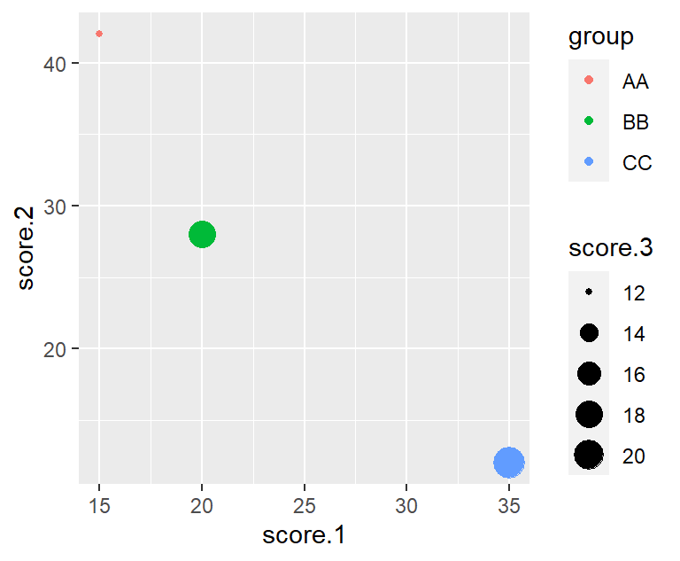

# Column Graph
#   Data: d.tbl
#   Geometry: column
#   Aesthetics: x, y, fill
#   Mapping: x=score.1, y=score.2, fill=score.3
ggplot(data=d.tbl, mapping=aes(x=score.1, y=score.2, fill=group)) + 
  geom_col()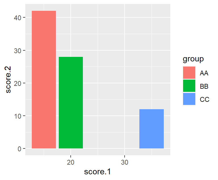

9.3.2 Geometries with required and optional aesthetics.

Geometry	Required aesthetics	Optional aesthetics
geom_abline()	slope, intercept	alpha, color, linetype, size
geom_hline()	yintercept	alpha, color, linetype, size
geom_vline()	xintercept	alpha, color, linetype, size
geom_area()	x, ymin, ymax	alpha, colour, fill, group, linetype, size
geom_col()	x, y	alpha, colour, fill, group, linetype, size
geom_bar()	x, y	alpha, colour, fill, group, linetype, size
geom_boxplot()	x, lower, middle, upper, ymax, ymin)	alpha, color, fill, group, linetype, shape, size, weight
geom_density()	x, y	alpha, color, fill, group, linetype, size, weight
geom_dotplot()	x, y	alpha, color, fill, group, linetype, stroke
geom_histogram()	x	alpha, color, fill, linetype, size, weight
geom_jitter()	x, y	alpha, color, fill, shape, size
geom_line()	x, y	alpha, color, linetype, size
geom_point()	x, y	alpha, color, fill, shape, size
geom_ribbon()	x, ymax, ymin	alpha, color, fill, linetype, size
geom_smooth()	x, y	alpha, color, fill, linetype, size, weight
geom_text()	label, x, y	alpha, angle, color, family, fontface, hjust, lineheight, size, vjust

9.3.3 Plot types

Figure 9.1: Plot types and geometries

9.3.4 Themes