1 How to use R

There are so many ways to analyse data in R. In my opinion the best way is the RStudio. Most R users use R via RStudio. We need both Base R and RStudio, as we did earlier, but if we only start the RStudio, so we can reach all functions of R. RStudio is an integrated development environment (IDE) that provides an interface by adding many convenient features and tools.

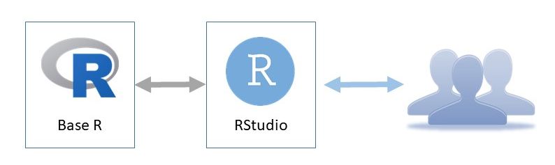
Figure 1.1: How to use R – the best way

Of course, we can use the Base R directly. Usually, this is the only option that is supported by mainframe environment. But, if you have the opportunity, always use RStudio instead of Basic R directly.

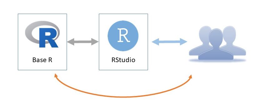
Figure 1.2: How to use R – the minimum way

Actually, there are several ways to use R, not only Base R and RStudio. The table below summarizes the interfaces in the columns and the tools in the rows. There are three different types of interface: Console, Script and Point and click. Interfaces allow the user to interact with R. 

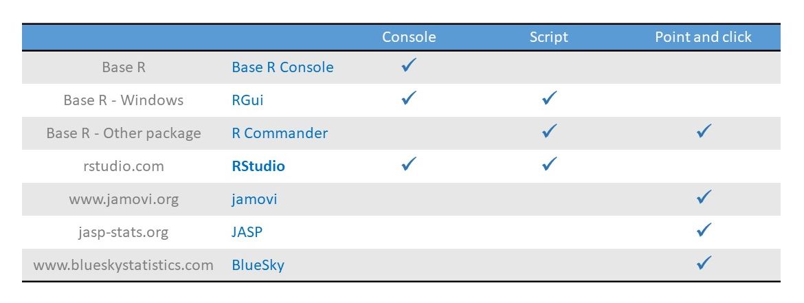
Figure 1.3: How to use R – the minimum way

Console provides a command-line interface that allows the user to interact with the computer by typing commands . The computer displays a prompt (>), the user types a command and presses Enter or Return, and gets the result. There are three tools, that provide console, the Base R Console (it’s the only option in mainframe environment), RGui in Base R on Windows, and RStudio.

The second interface is the script interface. It gives you an editor window. You can type multiple lines of code into the source editor without having each line evaluated by R. Then, when you’re ready, you can send the instructions to R - in other words, source the script -, and you get the result. You can reach this functionality in RGui, R Commander and RStudio. Remember, the best way to use R is creating, editing and running scripts in RStudio. This is the best option.

For beginners, the best option would be to use a Point-and-click interface. It has a menu, you can choose menupoints, menuitems, you can get dialog boxes and type in editfields, point on radio buttons and checkboxes. But the knowledge of these systems have limits. You can execute only methods, which you can reach from the menu. The descriptive measures, tables, plots and hypothesis tests, which you can point and click, are part of knowledge of R. The whole knowledge can be reached only from console or script interface. For example I only use jamovi, if I have a simple question and I want to get a quick answer.  So I encourage you to install and try jamovi or JASP. These are free and user friendly ways to do statistics. By the way, the tools I listed in this table are all free, except the BlueSky. It is worth installing and trying them.

1.1 Base R

What components were installed with Base R? The Base R consists of three elements. The console for typing commands and getting results, the interpreter for evaluating the commands, and packages for extending R’s knowledge. The interpreter is the heart of the R, all commands will be executed by the interpreter. For the users, for us, the console is the key. Apart from point and click interfaces, we will interact with the console directly or indirectly.

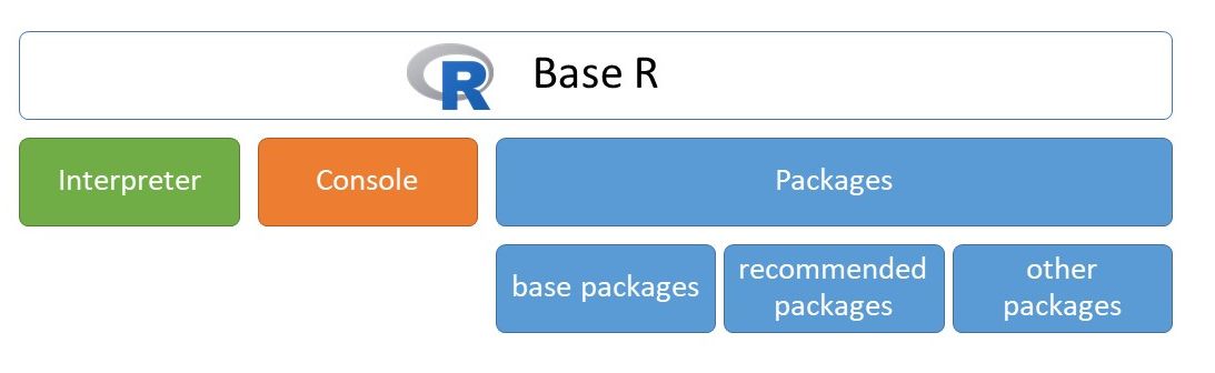
Figure 1.4: Components of Base R

1.1.1 Console of Base R

As we mentioned, the R users meet the console all the time. One main part of Base R is the console. To start the console, we should type R (the capital R letter) on all systems, or we can find and click on the R icon. If you are on Windows, you can launch the R.exe (e.g. c:\Program Files\R\R-4.0.4\bin\x64\R.exe).

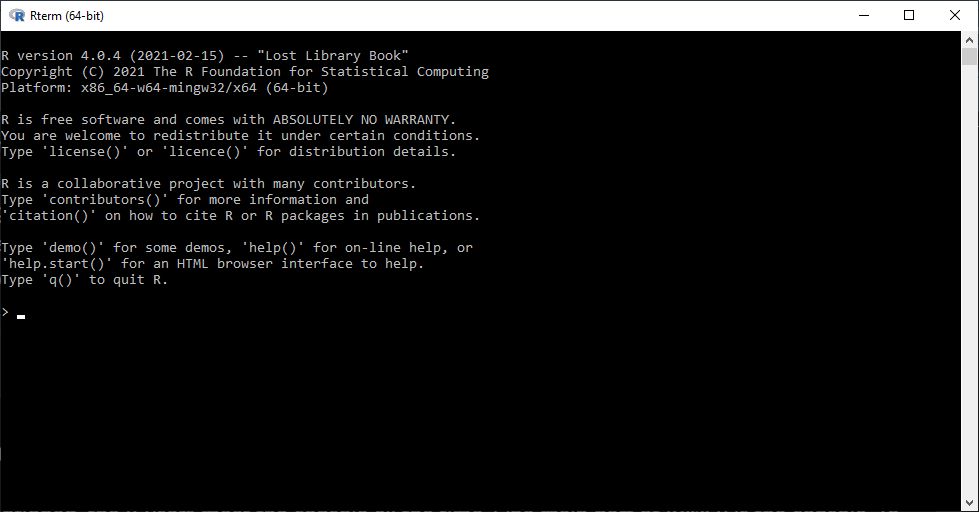
Figure 1.5: Console in Base R

On the screen above, you can see some information about the R instance. At the bottom of the console window there is a prompt. It consists of a ‘greater than’ sign (symbol) and a space, and of course a cursor where you can type any character.

Let’s type any character, delete characters with Delete and Backspace keys, move the cursor with Left arrow and Right arrow keys, insert any character in this position, and navigate the cursor the beginning of the line and the end of the line with the Home and End keys.

If we are ready, we can execute this line, the command, hitting Enter.

If the command is valid, R or more precisely its interpreter, will execute it, then it returns the result in the console. If the command in not valid, the interpreter returns an error message.

Let’s start with numbers. Type 45 and hit Enter.

45
#> [1] 45

This is a valid command because there is no error message. But the result, the output, is meaningless.

Let’s choose a more complicated expression:

45 + 5
#> [1] 50

Forty-five plus five sums fifty, so fifty is displayed in the output. The 1 in brackets at the beginning of the output means this is the first line of the output.

1.1.1.1 Console features

Every console has three features, that help us to execute commands.

History of commands

We can use the Up arrow and Down arrow keys to browse the history of commands, which we typed earlier. When you press the Up arrow, you get the commands you typed earlier at the command line. Of course you can modify them as well. You can hit Enter at any time to run the command that is currently displayed.

Autocompletion

Pressing TAB key completes the keyword or directory path we were currently typing. Type in getw hit TAB and you can see the whole function call, hitting Enter, you can get the working directory.

Continuation prompt

Let’s have a look at a small example. Tpye 45 -(forty-five minus) and hit Enter. This is an invalid command, but we can not see any Error message. Instead, a new prompt has appeared, a continuation prompt indicated by a + (plus) followed by a space character. We can continue typing. The console allows us to complete the command. It’s easy, type for example 5 (five), hit Enter. We can get the result. I’ll show you another example. Type getwd( without closing parenthesis, hit Enter. We will get the continuation prompt, and typing closing parenthesis we get the working directory. It seems to help us. Continuation prompt seems to be a good thing. But, It is not. It is a really confusing feature. We can easily find ourselves in a never ending story. We can type 45 -, Enter, 11 *, Enter and so on, we keep getting the continuation prompt, and we don’t really know how to complete it in a right way. So, It is very important to leave the continuation prompt as soon as possible. The key is Esc button. Lets’ try this. Type in opening parenthesis and 6 ((6), hit Enter, and press Esc. We can get back the prompt ‘greater than’ (>), this is default prompt. When you see the plus prompt, continuation prompt, you must press the Esc key.

1.1.1.2 Working directory

In R, we answer the questions we face using functions. So, the expressions that we type into the command line, usually contains function calls. So, now, we can request the working directory. Let’s type getwd() to get the interpreter to display our working directory.

getwd()

Working directory is the default directory that our command line reaches to access files if we don’t specify a path ourselves. We can specify paths two ways either absolutely from the root directory or relatively starting from our working directory. Beside reaching our history in the command line we can also rely on the help of a built-in autocompletion feature, by pressing TAB key, which completes the keyword or directory path we were currently typing.

For example, let’s type only set and press TAB and TAB again to list out all the commands that start with set. Press w and press TAB again, and as you can see the command line completes our command with a d to get an existing function name. All function call requires parentheses after the function name, which contains additional data for the function which we call arguments.

The setwd() function has only one required arguments, which is a path to a directory, which we want to set as our new working directory.

Let’s try calling the setwd() function, start with the function name, then the opening parenthesis and inside quote marks we give the directory’s path.

On Windows, after the first quote mark, type c:/, which refers the drive you want to use, and press TAB twice to see all subdirectories and files on the drive.

From here we can build our path directory by directory till we reach the directory which we want to set as our working directory. As you can see when jumping from directory into another we mark this jump with the slash character. Instead of writing out the path ourselves we can write the first few characters of directory’s name and we can rely on TAB to autocomplet it for us. Of course with more common directory names we have to be more specific to get the desired autocompletions.

Finally, if we reached our desired new working directory, we can execute the command, by pressing enter, but make sure you have both your opening and closing quote marks and parenthesis. If you had, your command executed successfully thereby changing your working directory, but if you made a mistake either in the formality of the command (called syntactic error) or by giving a path to a directory which doesn’t exist (called semantic error).

To sum up, to set a working directory in R type:

setwd("Path/To/Your/Workingdirectory")

If you need to check which working directory R thinks it is in:

getwd()

1.1.1.3 Quit the console

In the end, let’s quit the console, by typing and executing the q() command. Don’t forget the parentheses. We don’t need to save the workspace. Choose No.

1.1.2 RGui on Windows

On Windows operating system, Base R has another console which is more advanced. The RGui has a graphical user interface. To start it, find and click on the R icon. You should always use the latest version and the 64 bit version.

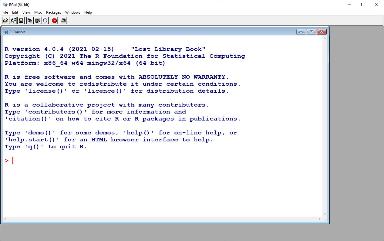
Figure 1.6: Console in RGui

Let’s start up the aforementioned 64 bit version of it. Above you can see our console which in functionality is the same as the one we used in Base R recently. We can type any character and press Enter.

If you’d like to change the appearance, or the size of the console, you can do so in the Edit > GUI preferences menu in the upper menu bar. Let’s choose this menu item, and increase the font size to 28 and set the style to bold. Close this dialog box with OK button, and you can see a more readable console window. But as you can see we also have menu and tool bar.

Let’s try the same basic arithmetic command here. Type 45 + 5 and press Enter to execute it. And as we can see we get the same result here.

Let’s try the history with the Up arrow and Down arrow. Navigate the cursor with Left arrow and Right arrow keys, use the Home and End buttons, insert or delete any character and press Enter.

1.1.2.1 Scripting in RGui

RGui has all the functions the Console of Base R had, and also a new one. We can create script files with which we can use to store commands in text files. Script files makes easy to store and organize commands. So let’s click File > New script which will make us a new script window where you can edit your script file. We can arrange the Console and Script windows, click on the Windows > Tile horizontally. You can find the typical face of RGui below.

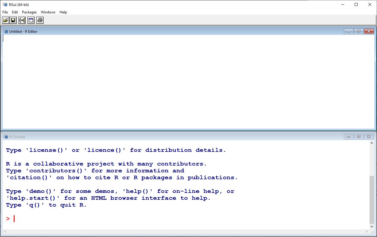
Figure 1.7: Console in RGui

Let’s write the two commands in to this script file: 45 + 5 and getwd().

Here we only type out command, to actually execute them we will need to transfer them to the console. This window is only a text editor through which we edit our script file. Here we can only use basic notepad like functionalities, so no autocompletion or history.

We can move in a line with the Home and End buttons and through lines with the Page Up and Page Down buttons. With Ctrl+Home we can get to the beginning of the script file and with Ctrl+End we can get to the bottom of it. Of course, this comes handy with much larger script files.

We can mark parts of the text with either holding the Shift key and using the Left-Right-Up-Down arrow keys or using the mouse. And we can use the clipboard as well, Ctrl+C, Ctrl+X and Ctrl+V.

It’s important to know how to actually execute the commands we just wrote into our script file. With Ctrl+R we can execute the line that our cursor is currently at. The process consists of the command getting pulled into the console and then it executing it.

Let’s try it. Move the cursor into the first line. Click in the first line anywhere. Then press the Ctrl+R. Three things happened at he same time. The first line was pulled into the console, the line was executed, and the cursor jumped down a line. We can repress the Ctrl+R and repeat the whole process for the second line. And so on.

If you have any text selected in your editor prior, pressing Ctrl+R, then the selected text will be executed. Let’s also try this. Select only 5 + 5 from the first line, and press Ctrl+R, and you get 10. Then, select the first two lines and execute them with Ctrl+R. The interpreter ran both lines. You can see the result in the console.

As you might have noticed, we have a colored console, the inputs, the commands colored by red, and the outputs, the results colored by blue.

This script files can also contain comments, which is useful to mark what’s the command’s intention. Which ones again may seem unimportant now, but is really useful when working with massive script files.

To mark something as a comment use the hash mark (#) which marks everything in a line after the hash mark as a comment. It’s good practice to start your script file with 3 comment lines which contains the author of the file, the date and a name which gives some kind of information about what the script does.

# Kálmán Abari
# 2021-03-17
# First script file

Navigate the cursor to the first position of the file, for example pressing the Ctrl+Home. Then type a hash mark, and your name, Enter. Hash mark, date of today, Enter, hash mark First script file, Enter.

If we are ready, we are going to save the script file. It’s important to save the script file with the File > Save menu. It’s good practice to save your work every 15 minutes. It’s important that when we save our files we give them names that doesn’t contain any special characters or whitespaces, underscores are acceptable though. Choose a proper directory and type in first_script.R as the filename. Make sure that our file’s extension should be .R which means that it contains an R script file.

With that we covered the basics of the RGui, so we can close it for now, we shouldn’t worry about saving our workspace since we won’t be needing it.

1.2 RStudio

The last tool we will get to know now and will be using for the rest of the book is RStudio. We can also launch it from the start menu. While we had multiple Basic R instances, we only have one RStudio, so it should be easy to find it.

It’s the most advanced interface to use R from the aforementioned ones. And this will be the one that we will mainly use through out the course. Even though we will only use RStudio, it’s important to mention that RStudio relies on Base R to work.

1.2.1 Customization

We can easily check which instance of Base R our RStudio is using. We can see this in the Global options > Tools menu option.

Let’s check if it really is using the 64 bit version.

Here we can also do other customizations. While we’re here we should also uncheck the Restore .Rdata option and set the Save workspace to Rdata on exit option to Never.

Another important one is the Code menu point from the left list. Here under the Saving option we have to set the Default text encoding to UTF-8 which is a wildly used and accepted character-code standard.

You can customize to look of your editor under the Appearance option. Here you can change the theme of your editor, which is sets the color palette it uses. I recommend changing it to Tomorrow night bright. Let’s close the settings, by pressing OK, to save the changes we made.

1.2.2 Using RStudio

A few words about RStudio. The main area consists of 3 or 4 different panes or windows which all are responsible for a different task. You have 3 panes by basic. The fourth panes you can add is a script file editor, which you can do by creating a new script file in File > New file >-- R Script.

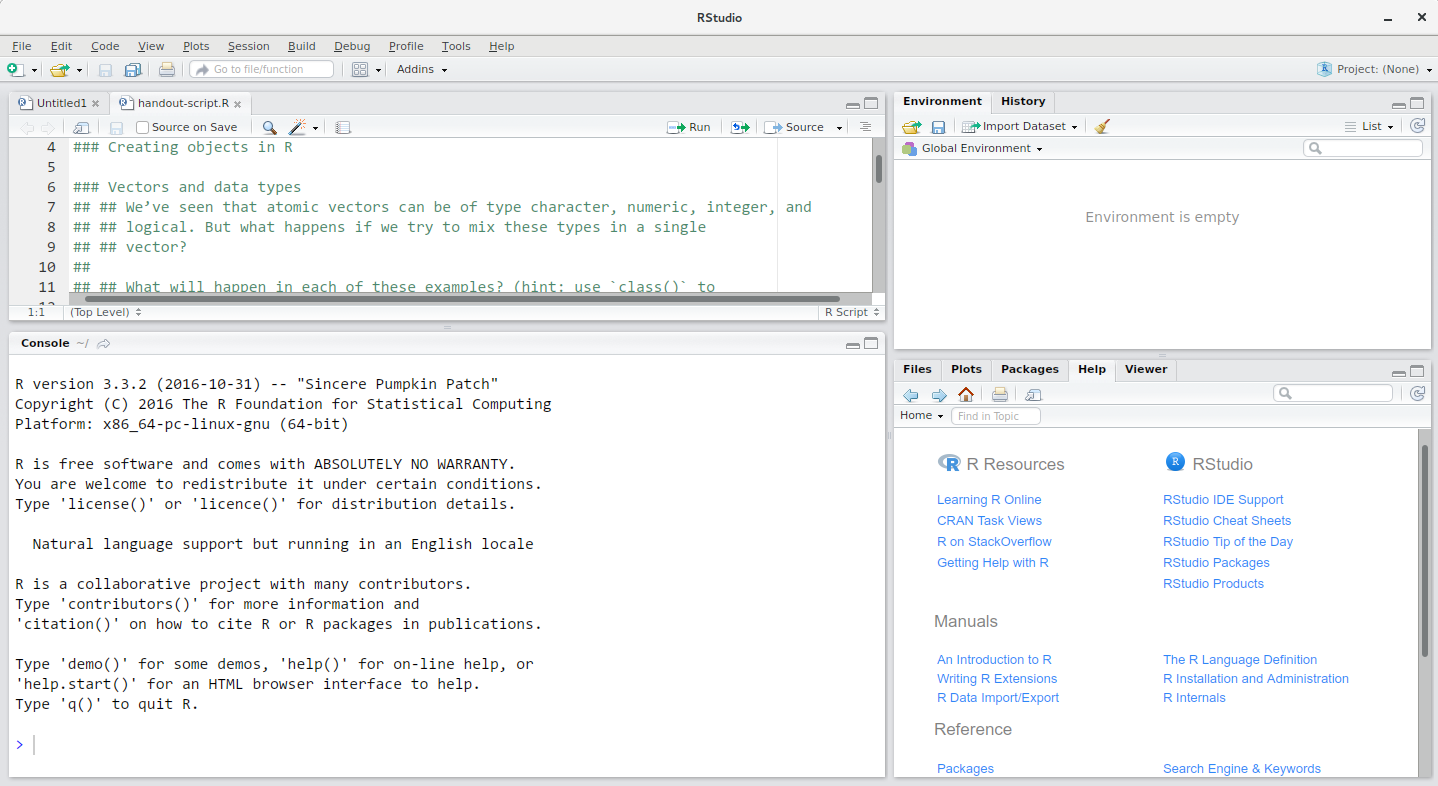
Figure 1.8: The RStudio Interface

You can easily resize the panes with clicking and dragging the vertical or horizontal line between the panes.

RStudio is divided into 4 “Panes”:

• the Source for your scripts and documents (top-left, in the default layout),
• the R Console (bottom-left),
• your Environment/History (top-right), and
• your Files/Plots/Packages/Help/Viewer (bottom-right).

The placement of these panes and their content can be customized (see main Menu Tools > Global Options > Pane Layout. One of the advantages of using RStudio is that all the information you need to write code is available in a single window.

1.2.3 How to start an R project

It is good practice to keep a set of related data, analyses, and text self-contained in a single folder. When working with R and RStudio you typically want that single top folder to be the folder you are working in. In order to tell R this, you will want to set that folder as your working directory. Whenever you refer to other scripts or data or directories contained within the working directory you can then use relative paths to files that indicate where inside the project a file is located. (That is opposed to absolute paths, which point to where a file is on a specific computer). Having everything contained in a single directory makes it a lot easier to move your project around on your computer and share it with others without worrying about whether or not the underlying scripts will still work.

Whenever you create a project with RStudio it creates a working directory for you and remembers its location (allowing you to quickly navigate to it) and optionally preserves custom settings and open files to make it easier to resume work after a break. Below, we will go through the steps for creating an “R Project” for this workshop.

• Start RStudio
• Under the File menu, click on New project, choose New directory, then Empty project
• As directory (or folder) name enter r-intro and create project as subdirectory of your desktop folder: ~/Desktop
• Click on Create project
• Under the Files tab on the right of the screen, click on New Folder and create a folder named data within your newly created working directory (e.g., ~/r-intro/data)
• On the main menu go to Files > New File > R Script (or use the shortcut Ctrl+Shift+N) to open a new file
• Save the empty script as r-intro-script.R in your working directory.

Your working directory should now look like in Figure 1.9.

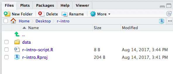
Figure 1.9: What it should look like at the beginning of this lesson

1.2.4 Organizing your working directory

Using a consistent folder structure across your projects will help keep things organized, and will also make it easy to find/file things in the future. This can be especially helpful when you have multiple projects. In general, you may create directories (folders) for data, documents, and outputs.

• data/ Use this folder to store your raw input data.
• documents/ If you are working on a paper this would be a place to keep outlines, drafts, and other text.
• output/ Use this folder to store your intermediate or final datasets and images you may create for the need of a particular analysis. For the sake of transparency, you should always keep a copy of your raw data accessible and do as much of your data cleanup and preprocessing programmatically, You could have subfolders in your output directory named output/data that would contain the respective processed files. I also like to save my images in output/image directory.

You may want additional directories or subdirectories depending on your project needs, but this is a good template to form the backbone of your working directory.

1.2.5 RStudio Console and Command Prompt

The console pane in RStudio is the place where commands written in the R language can be typed and executed immediately by the computer. It is also where the results will be shown for commands that have been executed. You can type commands directly into the console and press Enter to execute those commands, but they will be forgotten when you close the session.

If R is ready to accept commands, the R console by default shows a > prompt. If it receives a command (by typing, copy-pasting or sent from the script editor using Ctrl Enter), R will try to execute it, and when ready, will show the results and come back with a new > prompt to wait for new commands.

If R is still waiting for you to enter more data because it isn’t complete yet, the console will show a + prompt. It means that you haven’t finished entering a complete command. This is because you have not ‘closed’ a parenthesis or quotation, i.e. you don’t have the same number of left-parentheses as right-parentheses, or the same number of opening and closing quotation marks. When this happens, and you thought you finished typing your command, click inside the console window and press Esc; this will cancel the incomplete command and return you to the > prompt.

1.2.6 RStudio Script Editor

Because we want to keep our code and workflow, it is better to type the commands we want in the script editor, and save the script. This way, there is a complete record of what we did, and anyone (including our future selves!) can easily replicate the results on their computer.

Perhaps one of the most important aspects of making your code comprehensible for others and your future self is adding comments about why you did something. You can write comments directly in your script, and tell R not no execute those words simply by putting a hashtag (#) before you start typing the comment.

# this is a comment on its on line
getwd() # comments can also go here

One of the first things you will notice is in the R script editor that your code is colored (syntax coloring) which enhances readability.

Secondly, RStudio allows you to execute commands directly from the script editor by using the Ctrl + Enter shortcut (on Macs, Cmd + Enter will work, too). The command on the current line in the script (indicated by the cursor) or all of the commands in the currently selected text will be sent to the console and executed when you press Ctrl + Enter. You can find other keyboard shortcuts under Tools > Keyboard Shortcuts Help (or Alt + Shift + K)

At some point in your analysis you may want to check the content of a variable or the structure of an object, without necessarily keeping a record of it in your script. You can type these commands and execute them directly in the console. RStudio provides the Ctrl + 1 and Ctrl + 2 shortcuts allow you to jump between the script and the console panes.

All in all, RStudio is designed to make your coding easier and less error-prone.

1.3 RMarkdown

1.3.1 Introduction

RMarkdown allows you write reports that include both R codes and the output generated. Moreover, these reports are dynamic in the sense that changing the data and reprocessing the file will result in a new report with updated output. RMarkdown also lets you include Latex math, hyperlinks and images. These dynamic reports can be saved as

• PDF or PostScript documents
• Web pages
• Microsoft Word documents
• Open Document files
• and more like Beamer slides, etc.

When you render an RMarkdown file, it will appear, by default, as an HTML document in Viewer window of RStudio. If you want to create PDF documents, install a LaTeX compiler. Install MacTeX for Macs (http:// tug.org/mactex), MiKTeX (www.miktex.org) for Windows, and TeX Live for Linux (www.tug.org/texlive). Alternatively, you can install TinyTeX from https://yihui.name/tinytex/.

1.3.2 Basic Structure of R Markdown

Let’s start with a simple RMarkdown file and see what it looks like and the output that it produces when executed. Click File > New File > R Markdown, type in the title Homework problems, and the author. Click OK. Save the file with Ctrl+S, choose a name for example, homework_1.Rmd.

Rmarkdown files ends with the .Rmd extension. An .Rmd file contains three types of contents:

1. A YAML header :

---
title: "Homework problems"
author: "Abari Kálmán"
date: '2021 03 31 '
output: html_document
---

YAML stands for “yet another markup language” (https://en.wikipedia.org/wiki/YAML).

2. R code chuncks. For example:

```{r}
myDataFrame <- data.frame(names = LETTERS[1:3], variable_1 = runif(3))
myDataFrame
```

3. Text with formatting like bold text, mathematical expressions (), or headings # Heading, etc.

First let’s see how we can execute an .Rmd file to produce the output as PDF, HTML, etc.

Now click Knit to produce a complete report containing all text, code, and results. Alternatively, pressing Ctrl+Shift+K renders the whole document. But in this case, all output formats that are specified in the YAML header will be produced. On the other hand, Knit allows you to specify the output format you want to produce. For example, Knit > Knit to HTML produces only HTML output, which is usually faster than producing PDF output.

You can also render the file programmatically with the following command:

rmarkdown::render("homework_1.Rmd") 

This will display the report in the viewer pane, and create a self-contained HTML file.

Instead of running the whole document, you can run each individual code chunk by clicking the Run icon at the top right of the chunk or by pressing Ctrl+Shift+Enter. RStudio executes the code and displays the results inline with the code.

1.3.3 Text Formatting with R Markdown

This section demonstrates the syntax of common components of a document written in R Markdown. Inline text will be italic if surrounded by underscores or asterisks, e.g., _text_ or *text*. Bold text is produced using a pair of double asterisks (**text**). A pair of tildes (~) turn text to a subscript (e.g., H~3~PO~4~ renders H₃PO₄). A pair of carets (^) produce a superscript (e.g., Cu^2+^ renders Cu²⁺).

Hyperlinks are created using the syntax [text](link), e.g., [RStudio](https://www.rstudio.com). The syntax for images is similar: just add an exclamation mark, e.g., ![alt text or image title](path/to/image). Footnotes are put inside the square brackets after a caret ^[], e.g., ^[This is a footnote.].

Section headers can be written after a number of pound signs, e.g.,

# First-level header

## Second-level header

### Third-level header

If you do not want a certain heading to be numbered, you can add {-} or {.unnumbered} after the heading, e.g.,

# Preface {-}

Unordered list items start with *, -, or +, and you can nest one list within another list by indenting the sub-list, e.g.,

- one item
- one item
- one item
    - one more item
    - one more item
    - one more item

The output is:

• one item

• one item

• one item

  • one more item
  • one more item
  • one more item

Ordered list items start with numbers (you can also nest lists within lists), e.g.,

1. the first item
2. the second item
3. the third item
    - one unordered item
    - one unordered item

The output does not look too much different with the Markdown source:

1. the first item

2. the second item

3. the third item

   • one unordered item
   • one unordered item

Blockquotes are written after >, e.g.,

> "I thoroughly disapprove of duels. If a man should challenge me,
  I would take him kindly and forgivingly by the hand and lead him
  to a quiet place and kill him."
>
> --- Mark Twain

The actual output (we customized the style for blockquotes in this book):

“I thoroughly disapprove of duels. If a man should challenge me, I would take him kindly and forgivingly by the hand and lead him to a quiet place and kill him.”

— Mark Twain

Plain code blocks can be written after three or more backticks, and you can also indent the blocks by four spaces, e.g.,

```
This text is displayed verbatim / preformatted
```

Or indent by four spaces:

    This text is displayed verbatim / preformatted

In general, you’d better leave at least one empty line between adjacent but different elements, e.g., a header and a paragraph. This is to avoid ambiguity to the Markdown renderer. For example, does “#” indicate a header below?

In R, the character
# indicates a comment.

And does “-” mean a bullet point below?

The result of 5
- 3 is 2.

Different flavors of Markdown may produce different results if there are no blank lines.

1.3.4 Math expressions

Inline LaTeX equations can be written in a pair of dollar signs using the LaTeX syntax, e.g., $f(k) = {n \choose k} p^{k} (1-p)^{n-k}$ (actual output: \(f(k)={n \choose k}p^{k}(1-p)^{n-k}\)); math expressions of the display style can be written in a pair of double dollar signs, e.g., $$f(k) = {n \choose k} p^{k} (1-p)^{n-k}$$, and the output looks like this:

\[f\left(k\right)=\binom{n}{k}p^k\left(1-p\right)^{n-k}\]

You can also use math environments inside $ $ or $$ $$, e.g.,

$$\begin{array}{ccc}
x_{11} & x_{12} & x_{13}\\
x_{21} & x_{22} & x_{23}
\end{array}$$

\[\begin{array}{ccc} x_{11} & x_{12} & x_{13}\\ x_{21} & x_{22} & x_{23} \end{array}\]

$$X = \begin{bmatrix}1 & x_{1}\\
1 & x_{2}\\
1 & x_{3}
\end{bmatrix}$$

\[X = \begin{bmatrix}1 & x_{1}\\ 1 & x_{2}\\ 1 & x_{3} \end{bmatrix}\]

$$\Theta = \begin{pmatrix}\alpha & \beta\\
\gamma & \delta
\end{pmatrix}$$

\[\Theta = \begin{pmatrix}\alpha & \beta\\ \gamma & \delta \end{pmatrix}\]

$$\begin{vmatrix}a & b\\
c & d
\end{vmatrix}=ad-bc$$

\[\begin{vmatrix}a & b\\ c & d \end{vmatrix}=ad-bc\]