3 Getting started with a data analysis
3.1 Terminology
Before we begin data management tasks, we need a few vocabulary terms would be useful to discuss. Data scientists were usually interested in the characteristics and behaviors of humans and organizations. To understand these things, scientists often measured and recorded information about people or organizations.
Dataset 1 - Marijuana legalization
For example, a data scientist working on social science might be interested in understanding whether age is related to votes for marijuana legalization. To get this information, in several years, including 2016, the GSS survey included a question asking the survey participants whether they support marijuana legalization.
The GSS question was worded as follows:
- Do you think the use of marijuana should be legal or not?
Below the question, the different response options were listed:
- legal,
- not legal,
- don’t know (
DK), - no answer (
NA), - not applicable (
IAP).
The GSS Data Explorer (https://gssdataexplorer.norc.org) allows people to create a free account and browse the data that have been collected in the surveys. We used the Data Explorer to select the marijuana legalization question and a question about age. The age is important, since marijuana legalization had been primarily up to voters so far, the success of ballot initiatives in the future will depend on the support of people of voting age. If younger people are more supportive, this suggests that over time, the electorate will become more supportive as the old electorate decreases.
We saved age and vote data from the GSS and made the data file with the
file name legal_weed_age_GSS2016_ch1.csv. You can see the first 6 rows
from this data file:
| grass | age |
|---|---|
| IAP | 47 |
| LEGAL | 61 |
| NOT LEGAL | 72 |
| IAP | 43 |
| LEGAL | 55 |
| LEGAL | 53 |
As you can see, each person is an observation, and there are two variables, voting behavior (grass) and age. In a typical dataset, observations are the rows and variables are the columns.
Example 2 - Student survey
Another example a data frame contains the responses of 237 Statistics I. students at the University of Adelaide to a number of questions. It contains a lot of variables:
Sex- The sex of the student. (Factor with levels “Male” and “Female.”)Wr.Hnd- span (distance from tip of thumb to tip of little finger of spread hand) of writing hand, in centimetres.NW.Hnd- span of non-writing hand.W.Hnd- writing hand of student. (Factor, with levels “Left” and “Right.”)Fold- “Fold your arms! Which is on top” (Factor, with levels “R on L,” “L on R,” “Neither.”)Pulse- pulse rate of student (beats per minute).Clap- ‘Clap your hands! Which hand is on top?’ (Factor, with levels “Right,” “Left,” “Neither.”)Exer- how often the student exercises. (Factor, with levels “Freq” (frequently), “Some,” “None.”)Smoke- how much the student smokes. (Factor, levels “Heavy,” “Regul” (regularly), “Occas” (occasionally), “Never.”)Height- height of the student in centimetres.M.I- whether the student expressed height in imperial (feet/inches) or metric (centimetres/metres) units. (Factor, levels “Metric,” “Imperial.”)Age- age of the student in years.
| Sex | Wr.Hnd | NW.Hnd | W.Hnd | Fold | Pulse | Clap | Exer | Smoke | Height | M.I | Age |
|---|---|---|---|---|---|---|---|---|---|---|---|
| Female | 18.5 | 18.0 | Right | R on L | 92 | Left | Some | Never | 173.00 | Metric | 18.250 |
| Male | 19.5 | 20.5 | Left | R on L | 104 | Left | None | Regul | 177.80 | Imperial | 17.583 |
| Male | 18.0 | 13.3 | Right | L on R | 87 | Neither | None | Occas | NA | NA | 16.917 |
| Male | 18.8 | 18.9 | Right | R on L | NA | Neither | None | Never | 160.00 | Metric | 20.333 |
| Male | 20.0 | 20.0 | Right | Neither | 35 | Right | Some | Never | 165.00 | Metric | 23.667 |
| Female | 18.0 | 17.7 | Right | L on R | 64 | Right | Some | Never | 172.72 | Imperial | 21.000 |
In statistics data are organized in what we call a data matrix or dataset, where each row represents an observation or a case and each column represents a variable. If you ever use spreadsheets, for example an Excel spreadsheet, this representation should be familiar to you as well. There are two types of variables, numerical and categorical. Numerical, in other words, quantitative variables, take on numerical values. It is sensible to add, subtract, take averages, etc., with these values. Categorical, or qualitative variables, take on a limited number of distinct categories. These categories can be identified with numbers or labels, but it wouldn’t be sensible to do arithmetic operations with these values.
Numerical variables can further be categorized as continuous or discrete. Continuous numerical variables are usually measured, such as height, and they can take on any numerical value. While we tend to round our height when we record it, it’s actually measured on a continuous scale.
Discrete numerical variables are generally counted, such as the number of cars a house. These can only be whole, non-negative numbers.
Categorical variables that have ordered levels are called ordinal. Think about a survey question where you’re asked how satisfied you are with the customer service you received, and the options are “very unsatisfied,” “unsatisfied,” “neutral,” “satisfied,” or “very satisfied.” These levels have an inherent ordering, and hence the variable would be called ordinal. If the levels of a categorical variable do not have an inherent ordering to them, then the variable is simply called nominal.
These terms in statistics have a pair in R. Dataset corresponds to data frame. Variable corresponds to columns of data frame. Discrete variables must be an integer or double vector in R. Continuous variables must be an integer or double vector in R, as well. Nominal or ordinal variables must be factor in R.
To sum it up, study the list below.
Terms in statistics - terms in R - example :
Data matrix, dataset - data frame - marijuana legalization dataset and survey dataset
Variable - columns of data frame - each column of two dataset: grass, age, Sex, Wr.Hnd, etc.
numerical / quantitative
- discrete - integer or double vector - Pulse
- continuous - integer or double vector - age, Wr.Hnd, NW.Hnd, Height, Age
categorical / qualitative
- ordinal - factor - Exer, Smoke
- nominal - factor - grass, Sex, W.Hnd, Fold, Clap, M.I
3.2 Read and write data
R has an extensive range of functions to import many types of data files. For example, R can import data from from text files, from Microsoft Excel, from popular statistical packages, and from web sites.
3.2.1 Importing data from a delimited text file
You can import data from delimited text files using read.table(), a function that reads a file in table format and saves it as a data frame. Each row of the table appears as one line in the file. The syntax is
mydataframe <- read.table(file, options)where file is a delimited file and the options are parameters controlling how data is processed. The most common options are listed below:
header=- A logical value indicating whether the file contains the variable names in the first line.sep=- The delimiter separating data values. The default issep="", which denotes one or more spaces, tabs, new lines, or carriage returns. Usesep=","to read comma-delimited files,sep="\t"to read tab-delimited files, andsep=";"to read semicolon-delimited filesdec=- The character","or"."used in the file for decimal pointsquote=- Character(s) used to delimit strings that contain special characters. By default this is either double (") or single (') quotes.comment.char=- A character vector of length one containing a single character or an empty string. Use "" to turn off the interpretation of comments altogether.fileEncoding=- Character string for encoding name, e.g."UTF-8","UTF-8-BOM"or"latin2".
Consider a text file named legal_weed_age_GSS2016_ch1.csv containing voters’ response for marijuana legalization question and age. Each line of the file represents a student. The first line contains the variable names, separated with commas. Each subsequent line contains a voter’s information, also separated with commas. The first few lines of the file are as follows:
grass,age
IAP,47
LEGAL,61
NOT LEGAL,72
IAP,43
LEGAL,55
LEGAL,53
IAP,50
NOT LEGAL,23
The file can be imported into a data frame using the following code:
# read the GSS 2016 data
gss.2016 <- read.table(file = "data/legal_weed_age_GSS2016_ch1.csv",
                       header = T, sep = ",", fileEncoding = "UTF-8-BOM")
The results are as follows:
head(gss.2016) # first 6 rows
#>       grass age
#> 1       IAP  47
#> 2     LEGAL  61
#> 3 NOT LEGAL  72
#> 4       IAP  43
#> 5     LEGAL  55
#> 6     LEGAL  53
str(gss.2016)
#> 'data.frame':    2867 obs. of  2 variables:
#>  $ grass: chr  "IAP" "LEGAL" "NOT LEGAL" "IAP" ...
#>  $ age  : chr  "47" "61" "72" "43" ...
There are several interesting things to note about how the data is imported. By default, read.table() do not convert character variables to factors. You can suppress this behaviour in a number of ways. Including the option stringsAsFactors=TRUE turns off this behaviour for all character variables. The variable age is a character vector, which is not desirable. Age is a continuous variable, so it must be a numeric in R. We will discuss this issue in detail later.
3.2.2 Importing data from Excel
The best way to read an Excel file is to import Excel worksheets directly using the rio package. Be sure to download and install it before you first use it. Alternatively, export it to a comma-delimited file from Excel and import it into R using the method described earlier.
The rio package can be used to read, write, many file formats. The import() function imports a worksheet into a data frame. The simplest format is
import(file)where file= is the path to an Excel workbook.
Let’s import the student survey: imports the first worksheet from the workbook survey.xlsx stored on project data directory and saves it as the data frame survey.
library(rio)
survey <- import(file = "data/survey.xlsx")
The results are as follows:
head(survey) # first 6 rows
#>      Sex Wr.Hnd NW.Hnd W.Hnd    Fold Pulse    Clap Exer Smoke
#> 1 Female   18.5   18.0 Right  R on L    92    Left Some Never
#> 2   Male   19.5   20.5  Left  R on L   104    Left None Regul
#> 3   Male   18.0   13.3 Right  L on R    87 Neither None Occas
#> 4   Male   18.8   18.9 Right  R on L    NA Neither None Never
#> 5   Male   20.0   20.0 Right Neither    35   Right Some Never
#> 6 Female   18.0   17.7 Right  L on R    64   Right Some Never
#>   Height      M.I    Age
#> 1 173.00   Metric 18.250
#> 2 177.80 Imperial 17.583
#> 3     NA     <NA> 16.917
#> 4 160.00   Metric 20.333
#> 5 165.00   Metric 23.667
#> 6 172.72 Imperial 21.000
str(survey)
#> 'data.frame':    237 obs. of  12 variables:
#>  $ Sex   : chr  "Female" "Male" "Male" "Male" ...
#>  $ Wr.Hnd: num  18.5 19.5 18 18.8 20 18 17.7 17 20 18.5 ...
#>  $ NW.Hnd: num  18 20.5 13.3 18.9 20 17.7 17.7 17.3 19.5 18.5 ...
#>  $ W.Hnd : chr  "Right" "Left" "Right" "Right" ...
#>  $ Fold  : chr  "R on L" "R on L" "L on R" "R on L" ...
#>  $ Pulse : num  92 104 87 NA 35 64 83 74 72 90 ...
#>  $ Clap  : chr  "Left" "Left" "Neither" "Neither" ...
#>  $ Exer  : chr  "Some" "None" "None" "None" ...
#>  $ Smoke : chr  "Never" "Regul" "Occas" "Never" ...
#>  $ Height: num  173 178 NA 160 165 ...
#>  $ M.I   : chr  "Metric" "Imperial" NA "Metric" ...
#>  $ Age   : num  18.2 17.6 16.9 20.3 23.7 ...
As you can see, the variable Sex, W.Hnd, etc. are a character vectors, which is not desirable. They are a categorical variables, so they must be factors in R.
3.2.3 Exporting data from R
So far, we reviewed a wide range of methods for importing data into R. But sometimes you’ll want to go the other way - exporting data from R - so that data can be archived or imported into external applications. Now, you’ll learn how to output an R object to a delimited text file, an Excel spreadsheet, or a statistical application (such as SPSS, SAS, or Stata).
You can use the write.table() function to output an R object to a delimited text file. The format is
write.table(x, outfile, sep=delimiter, quote=TRUE, na="NA")where x is the object and outfile is the target file. For example, the statement
write.table(x = survey, file = "output/data/survey.txt", sep = "\t",
            dec = ",", row.names = FALSE, quote = FALSE)
saves the dataset survey to a tab-delimited file named survey.txt in the project output/data directory. Replacing sep="\t" with sep=";" saves the data in a semicolon-delimited file. By default, strings are enclosed in quotes ("") and missing values are written as NA. We will not print row names (row.names = FALSE) and quote (quote = FALSE) in the output text file.
The export() function in the rio package can be used to save an R data frame to an Excel workbook. For example, the statements
library(rio)
export(x = gss.2016, file = "output/data/gss.xlsx")
export the data frame gss.2016 to a worksheet (Sheet 1 by default) in an Excel workbook named gss.xlsx in the project output/data directory. By default, the variable names in the dataset are used to create column headings in the spreadsheet, and row names are placed in the first column of the spreadsheet. If gss.xlsx already exists, it’s overwritten.
The export() function in the rio package can be used to export a data frame to an external statistical application. For example, the code
library(rio)
export(x = survey, file = "output/data/survey.sav")
exports the data frame survey into an SPSS data file named survey.sav.
Please study carefully the following codes and outputs:
# Export (tab or semicolon) delimited text files with and withot encoding
write.table(x = survey, file = "output/data/survey.txt", sep = "\t",
            dec = ",", row.names = FALSE, quote = FALSE)
write.table(x = survey, file = "output/data/survey.csv", sep = ";",
            dec = ",", row.names = FALSE, quote = FALSE)
write.table(x = survey, file = "output/data/survey_utf-8.txt", sep = "\t",
            dec = ",", row.names = FALSE, quote = FALSE, fileEncoding = "UTF-8")
write.table(x = survey, file = "output/data/survey_latin2.txt", sep = "\t",
            dec = ",", row.names = FALSE, quote = FALSE, fileEncoding = "latin2")
write.table(x = survey, file = "output/data/survey_utf-8.csv", sep = ";",
            dec = ",", row.names = FALSE, quote = FALSE, fileEncoding = "UTF-8")
write.table(x = survey, file = "output/data/survey_latin2.csv", sep = ";",
            dec = ",", row.names = FALSE, quote = FALSE, fileEncoding = "latin2")

# Export Excel and SPSS files
library(rio)
export(x = survey, file = "output/data/survey.xlsx")
export(x = survey, file = "output/data/survey.sav")
export(x = gss.2016, file = "output/data/gss.xlsx")
export(x = gss.2016, file = "output/data/gss.sav")
3.3 Data manipulation
In the previous chapter, we covered a variety of methods for importing data into R. Unfortunately, getting your data in the rectangular arrangement of a matrix or data frame is only the first step in preparing it for analysis. In this early stage we try to get as much information as we can.
3.3.1 Get information
When working with (large) data frames, you must first develop a clear understanding of the structure and main elements of the data set. Therefore, it can often be useful to show only a small part of the entire data set. To do this in R, you can use the functions head() or tail(). The head() function shows the first part of the data frame. The tail() function shows the last part. Both functions print a top line called the header which contains the names of the different variables in the data set.
head(gss.2016)
#>       grass age
#> 1       IAP  47
#> 2     LEGAL  61
#> 3 NOT LEGAL  72
#> 4       IAP  43
#> 5     LEGAL  55
#> 6     LEGAL  53
tail(gss.2016, n = 3)
#>          grass age
#> 2865     LEGAL  87
#> 2866       IAP  55
#> 2867 NOT LEGAL  72
Another method to get a rapid overview of the data is the str() function. The str() function shows the structure of the data set.
str(gss.2016)
#> 'data.frame':    2867 obs. of  2 variables:
#>  $ grass: chr  "IAP" "LEGAL" "NOT LEGAL" "IAP" ...
#>  $ age  : chr  "47" "61" "72" "43" ...
For a data frame it gives the following information:
- The total number of observations (e.g. 2867 voters)
- The total number of variables (e.g. 2 variables)
- A full list of the variables names (
grass,age) - The data type of each variable (
chr) - The first observations
When you receive a new data frame, applying the str() function is often the first step. It is a great way to get more insight into the data set before deeper analysis.
Please study carefully the following codes and outputs:
str(gss.2016)        # Structure of an Arbitrary R Object
#> 'data.frame':    2867 obs. of  2 variables:
#>  $ grass: chr  "IAP" "LEGAL" "NOT LEGAL" "IAP" ...
#>  $ age  : chr  "47" "61" "72" "43" ...
head(gss.2016)       # Return the First Parts of an Object
#>       grass age
#> 1       IAP  47
#> 2     LEGAL  61
#> 3 NOT LEGAL  72
#> 4       IAP  43
#> 5     LEGAL  55
#> 6     LEGAL  53
dim(gss.2016)        # Dimensions of an Object
#> [1] 2867    2
ncol(gss.2016)       # The Number of Rows of a data frame
#> [1] 2
nrow(gss.2016)       # The Number of Columns of a data frame
#> [1] 2867
names(gss.2016)      # The Column Names of an Object
#> [1] "grass" "age"
typeof(gss.2016)     # Type of an Object
#> [1] "list"
class(gss.2016)      # Class of an Object
#> [1] "data.frame"
str(survey)
#> 'data.frame':    237 obs. of  12 variables:
#>  $ Sex   : chr  "Female" "Male" "Male" "Male" ...
#>  $ Wr.Hnd: num  18.5 19.5 18 18.8 20 18 17.7 17 20 18.5 ...
#>  $ NW.Hnd: num  18 20.5 13.3 18.9 20 17.7 17.7 17.3 19.5 18.5 ...
#>  $ W.Hnd : chr  "Right" "Left" "Right" "Right" ...
#>  $ Fold  : chr  "R on L" "R on L" "L on R" "R on L" ...
#>  $ Pulse : num  92 104 87 NA 35 64 83 74 72 90 ...
#>  $ Clap  : chr  "Left" "Left" "Neither" "Neither" ...
#>  $ Exer  : chr  "Some" "None" "None" "None" ...
#>  $ Smoke : chr  "Never" "Regul" "Occas" "Never" ...
#>  $ Height: num  173 178 NA 160 165 ...
#>  $ M.I   : chr  "Metric" "Imperial" NA "Metric" ...
#>  $ Age   : num  18.2 17.6 16.9 20.3 23.7 ...
head(survey)
#>      Sex Wr.Hnd NW.Hnd W.Hnd    Fold Pulse    Clap Exer Smoke
#> 1 Female   18.5   18.0 Right  R on L    92    Left Some Never
#> 2   Male   19.5   20.5  Left  R on L   104    Left None Regul
#> 3   Male   18.0   13.3 Right  L on R    87 Neither None Occas
#> 4   Male   18.8   18.9 Right  R on L    NA Neither None Never
#> 5   Male   20.0   20.0 Right Neither    35   Right Some Never
#> 6 Female   18.0   17.7 Right  L on R    64   Right Some Never
#>   Height      M.I    Age
#> 1 173.00   Metric 18.250
#> 2 177.80 Imperial 17.583
#> 3     NA     <NA> 16.917
#> 4 160.00   Metric 20.333
#> 5 165.00   Metric 23.667
#> 6 172.72 Imperial 21.000
dim(survey)
#> [1] 237  12
ncol(survey)
#> [1] 12
nrow(survey)
#> [1] 237
names(survey)
#>  [1] "Sex"    "Wr.Hnd" "NW.Hnd" "W.Hnd"  "Fold"   "Pulse"
#>  [7] "Clap"   "Exer"   "Smoke"  "Height" "M.I"    "Age"
typeof(survey)
#> [1] "list"
class(survey)
#> [1] "data.frame"
3.3.2 Data type conversions
As you have known, in R, you use numeric vectors to represent quantitative variables, and you use factors to represent categorical variables. In the data frame gss.2016, the variable grass is character vector, but it should be a factor. R provides a set of functions to identify an object’s data type and convert it to a different data type. You can use the function factor() to convert from character or numeric to factor.
str(gss.2016)                             # grass is character
#> 'data.frame':    2867 obs. of  2 variables:
#>  $ grass: chr  "IAP" "LEGAL" "NOT LEGAL" "IAP" ...
#>  $ age  : chr  "47" "61" "72" "43" ...
gss.2016$grass <- factor(gss.2016$grass)  # convert
str(gss.2016)                             # grass is factor
#> 'data.frame':    2867 obs. of  2 variables:
#>  $ grass: Factor w/ 4 levels "DK","IAP","LEGAL",..: 2 3 4 2 3 3 2 4 2 4 ...
#>  $ age  : chr  "47" "61" "72" "43" ...
The continuous variable age is also character, but it should be a numeric. What is the problem with age variable? Use the unique() and table() functions.
unique(gss.2016$age)
#>  [1] "47"          "61"          "72"          "43"
#>  [5] "55"          "53"          "50"          "23"
#>  [9] "45"          "71"          "33"          "86"
#> [13] "32"          "60"          "76"          "56"
#> [17] "62"          "31"          "58"          "37"
#> [21] "25"          "22"          "74"          "75"
#> [25] "68"          "46"          "35"          "59"
#> [29] "79"          "40"          "44"          "36"
#> [33] "70"          "28"          "20"          "41"
#> [37] "42"          "57"          "26"          "51"
#> [41] "39"          "27"          "30"          "29"
#> [45] "80"          "49"          "78"          "52"
#> [49] "66"          "89 OR OLDER" "54"          "48"
#> [53] "81"          "69"          "21"          "64"
#> [57] "38"          "65"          "67"          "84"
#> [61] "34"          "77"          "19"          NA
#> [65] "83"          "73"          "63"          "24"
#> [69] "82"          "85"          "87"          "18"
#> [73] "88"
table(gss.2016$age, useNA = "ifany")
#>
#>          18          19          20          21          22
#>           7          33          26          33          44
#>          23          24          25          26          27
#>          49          35          56          42          58
#>          28          29          30          31          32
#>          42          56          54          57          42
#>          33          34          35          36          37
#>          54          49          56          52          58
#>          38          39          40          41          42
#>          44          42          46          36          50
#>          43          44          45          46          47
#>          45          52          27          45          55
#>          48          49          50          51          52
#>          46          41          48          49          65
#>          53          54          55          56          57
#>          60          53          48          48          70
#>          58          59          60          61          62
#>          67          58          53          56          56
#>          63          64          65          66          67
#>          43          34          44          47          49
#>          68          69          70          71          72
#>          43          42          32          27          26
#>          73          74          75          76          77
#>          22          24          19          25          23
#>          78          79          80          81          82
#>          26          21          25          21          11
#>          83          84          85          86          87
#>          22          11          11          12           9
#>          88 89 OR OLDER        <NA>
#>           3          22          10
unique(x) returns an object of the same type of x, but with only one copy of each duplicated element. table(x) returns the same, plus the number of times a particular value of x occurs.
Age appears to be measured in years up to age 88, and then "89 OR OLDER" represents people who are 89 years old or older. Since "89 OR OLDER" can not be a number, trying to force the age variable with "89 OR OLDER" in it into a numeric variable would result in an error. Before converting age into a numeric variable, you should first recode anyone who has a value of "89 OR OLDER" to instead have a value 89.
gss.2016$age[gss.2016$age %in% "89 OR OLDER"] <- "89"  # recoding
gss.2016$age <- as.numeric(gss.2016$age)               # data type conversion
str(gss.2016)
#> 'data.frame':    2867 obs. of  2 variables:
#>  $ grass: Factor w/ 4 levels "DK","IAP","LEGAL",..: 2 3 4 2 3 3 2 4 2 4 ...
#>  $ age  : num  47 61 72 43 55 53 50 23 45 71 ...
By now, the data frame gss.2016 is in the desired structure.
What about the data frame survey? As we mentioned, there are a few variables, namely Sex, W.Hnd, Fold, Clap, Exer,Smoke, andM.I, that are categorical, so you need to convert to factor. We can use the factor() function:
survey$Sex <- factor(survey$Sex)
survey$W.Hnd <- factor(survey$W.Hnd)
survey$Fold <- factor(survey$Fold)
survey$Clap <- factor(survey$Clap)
survey$Exer <- factor(survey$Exer)
survey$Smoke <- factor(survey$Smoke)
survey$M.I <- factor(survey$M.I)
str(survey)
#> 'data.frame':    237 obs. of  12 variables:
#>  $ Sex   : Factor w/ 2 levels "Female","Male": 1 2 2 2 2 1 2 1 2 2 ...
#>  $ Wr.Hnd: num  18.5 19.5 18 18.8 20 18 17.7 17 20 18.5 ...
#>  $ NW.Hnd: num  18 20.5 13.3 18.9 20 17.7 17.7 17.3 19.5 18.5 ...
#>  $ W.Hnd : Factor w/ 2 levels "Left","Right": 2 1 2 2 2 2 2 2 2 2 ...
#>  $ Fold  : Factor w/ 3 levels "L on R","Neither",..: 3 3 1 3 2 1 1 3 3 3 ...
#>  $ Pulse : num  92 104 87 NA 35 64 83 74 72 90 ...
#>  $ Clap  : Factor w/ 3 levels "Left","Neither",..: 1 1 2 2 3 3 3 3 3 3 ...
#>  $ Exer  : Factor w/ 3 levels "Freq","None",..: 3 2 2 2 3 3 1 1 3 3 ...
#>  $ Smoke : Factor w/ 4 levels "Heavy","Never",..: 2 4 3 2 2 2 2 2 2 2 ...
#>  $ Height: num  173 178 NA 160 165 ...
#>  $ M.I   : Factor w/ 2 levels "Imperial","Metric": 2 1 NA 2 2 1 1 2 2 2 ...
#>  $ Age   : num  18.2 17.6 16.9 20.3 23.7 ...
Our dataset survey contains only numeric and factor variables. But two variables (Exer anSmoke) are ordinal categorical variable, so you need to check the levels.
Sometimes it’s useful to know the number of levels of a factor. The convenience function nlevels() extracts the number of levels from a factor:
nlevels(survey$Exer)
#> [1] 3
To look at the levels of a factor, you use the levels() function. For example,
to extract the factor levels of Exer, use the following:
levels(survey$Exer)
#> [1] "Freq" "None" "Some"
As you can see, each student has a status of exercise (None, Some, Freq), how often the student exercises. Notice, in the output above the levels are ordered alphabetically. However, we need to sort in the order None, Some, Freq:
survey$Exer <- factor(survey$Exer, levels=c("None", "Some", "Freq"))
levels(survey$Exer)
#> [1] "None" "Some" "Freq"
In R, there is a really big practical advantage to order factor’s level. A great many R functions recognize and treat ordered factors differently by printing results in the order that you expect. For example,
table(survey$Exer, useNA = "ifany")
#>
#> None Some Freq
#>   24   98  115
We need to order the levels in Smoke variable.
levels(survey$Smoke)
#> [1] "Heavy" "Never" "Occas" "Regul"
table(survey$Smoke, useNA = "ifany")
#>
#> Heavy Never Occas Regul  <NA>
#>    11   189    19    17     1
survey$Smoke <- factor(survey$Smoke, levels=c("Never", "Occas", "Regul","Heavy"))
levels(survey$Smoke)
#> [1] "Never" "Occas" "Regul" "Heavy"
table(survey$Smoke, useNA = "ifany")
#>
#> Never Occas Regul Heavy  <NA>
#>   189    19    17    11     1
3.3.3 Transformation
3.3.4 Identifying and treating missing values
In addition to making sure the variables used are an appropriate type, it was also important to make sure that missing values were treated appropriately by R. In R, missing values are recorded as NA, which stands for not available. Researchers code missing values in many different ways when collecting and storing data. Some of the more common ways to denote missing values are the following:
- blank
- 777, -777, 888, -888, 999, -999, or something similar
- a single period
- -1
- NULL.
Other responses, such as “Don’t know” or “Inapplicable,” may sometimes be treated as missing or as response categories depending on what is most appropriate given the characteristics of the data and the analysis goals.
In the summary of the gss.2016 data,
summary(gss.2016)
#> grass age
#> DK : 110 Min. :18.00
#> IAP : 911 1st Qu.:34.00
#> LEGAL :1126 Median :49.00
#> NOT LEGAL: 717 Mean :49.16
#> NA's : 3 3rd Qu.:62.00
#> Max. :89.00
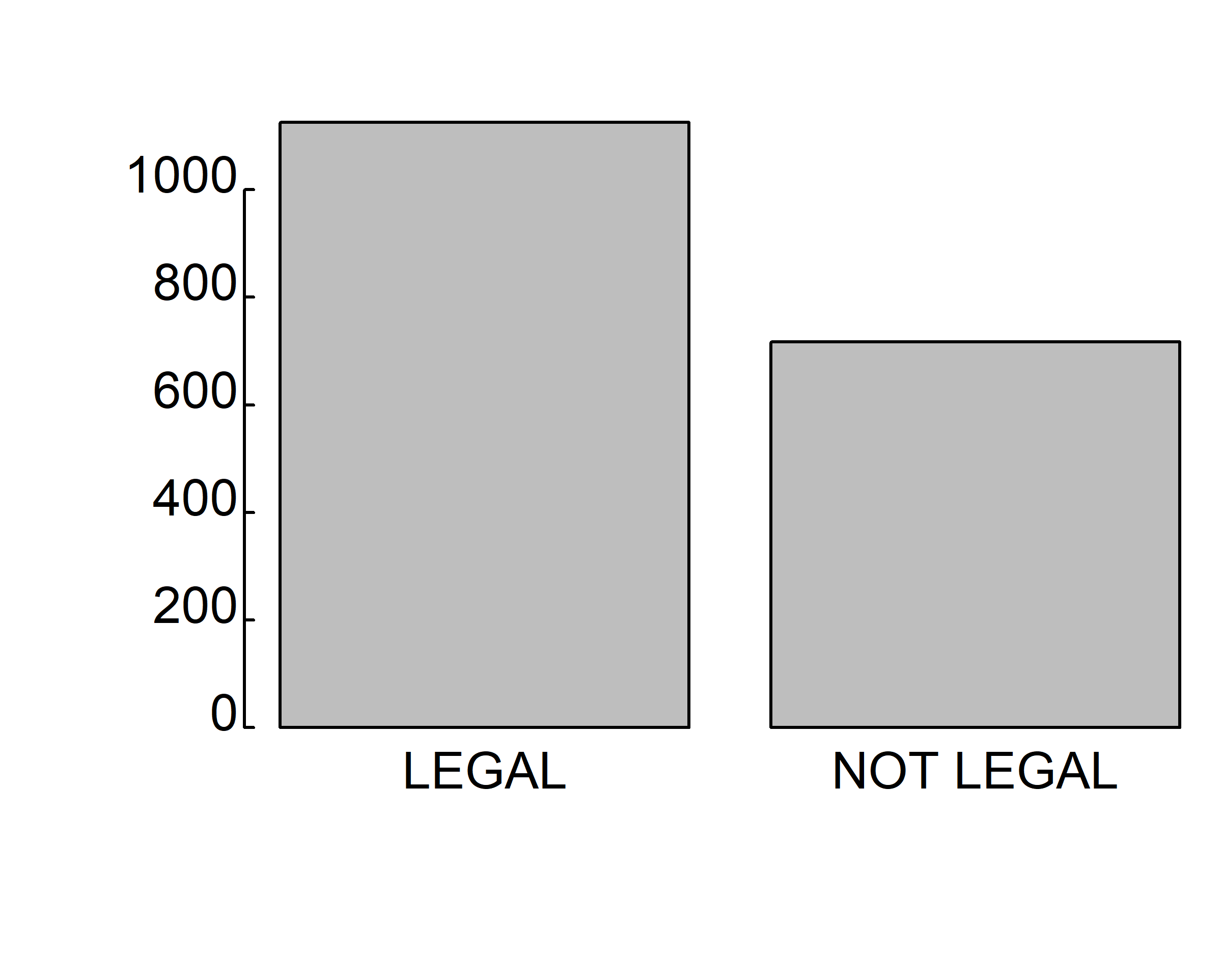
#> NA's :10the grass variable has five possible values: DK (don’t know), IAP (inapplicable), LEGAL, NOT LEGAL, and NA (not available). The DK, IAP, and NA could all be considered missing values. However, R treats only NA as missing. Before conducting any analyses, the DK and IAP values could be converted to NA to be treated as missing in any analyses. That is, the grass variable could be recoded so that these values are all NA. Note that NA is a reserved “word” in R. In order to use NA, both letters must be uppercase (Na or na does not work), and there can be no quotation marks (R will treat "NA" as a character rather than a true missing value). There are many ways to recode variables in R. For example,
table(gss.2016$grass, useNA = "ifany")   # before recoding
#>
#>        DK       IAP     LEGAL NOT LEGAL      <NA>
#>       110       911      1126       717         3
library(car)
gss.2016$grass <- car::recode(var = gss.2016$grass, recodes = 'c("DK", "IAP")=NA')
table(gss.2016$grass, useNA = "ifany")   # after recoding
#>
#>     LEGAL NOT LEGAL      <NA>
#>      1126       717      1024
3.3.5 Numeric to factor
In addition to solving the age and grass recoding, the final plan to create the age categories shown below. The age variable currently holds the age in years rather than age categories. The age can be in four categories:
- 18-29
- 30-59
- 60-74
- 75+
The function cut() can be used to divide a continuous variable into categories by cutting it into pieces and adding a label to each piece.
gss.2016$age.f <- cut(x = gss.2016$age, breaks = c(-Inf, 29, 59, 74, Inf),
    labels = c("<30", "30-59", "60-74", "75+" ))
table(gss.2016$age.f, useNA = "ifany")
#>
#>   <30 30-59 60-74   75+  <NA>
#>   481  1517   598   261    10
cut() takes a variable like age as the first argument. The second thing to add after the variable name is a vector made up of the breaks. Breaks specify the lower and upper limit of each category of values. The first entry is the lowest value of the first category, the second entry is the highest value of the first category, the third entry is the highest value of the second category, and so on. The first and last values in the vector are -Inf and Inf. These are negative infinity and positive infinity. This was for convenience rather than looking up the smallest and largest values of variable age. It also makes the code more flexible in case there is a new data point with a smaller or larger value. The final thing to add is a vector made up of the labels for the categories, with each label inside quote marks.
3.4 Descriptive statistics
R has built in functions for a large number of summary statistics. To illustrate the main R functions we will use the survey and gss.2016 datasets. R has tons of packages to explore our dataset, but we focus on built-in possibilities, psych and DescTools packages.
Let us first see what kind of objects are included in survey and gss.2016 by using summary() function.
summary(gss.2016)
#>        grass           age          age.f
#>  LEGAL    :1126   Min.   :18.00   <30  : 481
#>  NOT LEGAL: 717   1st Qu.:34.00   30-59:1517
#>  NA's     :1024   Median :49.00   60-74: 598
#>                   Mean   :49.16   75+  : 261
#>                   3rd Qu.:62.00   NA's :  10
#>                   Max.   :89.00
#>                   NA's   :10
summary(survey)
#>      Sex          Wr.Hnd          NW.Hnd        W.Hnd
#>  Female:118   Min.   :13.00   Min.   :12.50   Left : 18
#>  Male  :118   1st Qu.:17.50   1st Qu.:17.50   Right:218
#>  NA's  :  1   Median :18.50   Median :18.50   NA's :  1
#>               Mean   :18.67   Mean   :18.58
#>               3rd Qu.:19.80   3rd Qu.:19.73
#>               Max.   :23.20   Max.   :23.50
#>               NA's   :1       NA's   :1
#>       Fold         Pulse             Clap       Exer
#>  L on R : 99   Min.   : 35.00   Left   : 39   None: 24
#>  Neither: 18   1st Qu.: 66.00   Neither: 50   Some: 98
#>  R on L :120   Median : 72.50   Right  :147   Freq:115
#>                Mean   : 74.15   NA's   :  1
#>                3rd Qu.: 80.00
#>                Max.   :104.00
#>                NA's   :45
#>    Smoke         Height            M.I           Age
#>  Never:189   Min.   :150.0   Imperial: 68   Min.   :16.75
#>  Occas: 19   1st Qu.:165.0   Metric  :141   1st Qu.:17.67
#>  Regul: 17   Median :171.0   NA's    : 28   Median :18.58
#>  Heavy: 11   Mean   :172.4                  Mean   :20.37
#>  NA's :  1   3rd Qu.:180.0                  3rd Qu.:20.17
#>              Max.   :200.0                  Max.   :73.00
#>              NA's   :28
The type of the descriptive statistics we use depends on whether data is numeric (continuous) or categorical and so we will look at each case separately next.
3.4.1 Measurements
Recall that for numeric variables, we are usually interested in measuring center tendency and spread to get a sense of data. Suppose that we are interested in Height column, in which students’ height is measured. From the summary(survey) table above we know that this variable is indeed a numeric data, and therefore we can measure central tendency and spread of this variable as we do in the following codes, respectively:
# Central Tendency
mean(survey$Height, na.rm = T)     # Mean
#> [1] 172.3809
median(survey$Height, na.rm = T)   # Median
#> [1] 171

# Spread
min(survey$Height, na.rm = T)      # Minimum
#> [1] 150
max(survey$Height, na.rm = T)      # Maximum
#> [1] 200
range(survey$Height, na.rm = T)    # Range
#> [1] 150 200
IQR(survey$Height, na.rm = T)      # IQR
#> [1] 15
var(survey$Height, na.rm = T)      # Variance
#> [1] 96.9738
sd(survey$Height, na.rm = T)       # Standard Deviation
#> [1] 9.847528
All of these functions have optional arguments to address various complications that your data might have. For example, if your data includes some NAs, then instead of using mean(survey$Height) you should use mean(survey$Height, na.rm = T), which tells R to ignore NAs in the data.
Please study carefully the following codes and outputs:
#install.packages("psych")
library(psych)
describe(gss.2016)
#>        vars    n  mean    sd median trimmed   mad min max range
#> grass*    1 1843  1.39  0.49      1    1.36  0.00   1   2     1
#> age       2 2857 49.16 17.69     49   48.62 20.76  18  89    71
#> age.f*    3 2857  2.22  0.83      2    2.17  0.00   1   4     3
#>        skew kurtosis   se
#> grass* 0.45    -1.79 0.01
#> age    0.17    -0.90 0.33
#> age.f* 0.51    -0.16 0.02
describe(survey)
#>        vars   n   mean    sd median trimmed   mad    min   max
#> Sex*      1 236   1.50  0.50   1.50    1.50  0.74   1.00   2.0
#> Wr.Hnd    2 236  18.67  1.88  18.50   18.61  1.48  13.00  23.2
#> NW.Hnd    3 236  18.58  1.97  18.50   18.55  1.63  12.50  23.5
#> W.Hnd*    4 236   1.92  0.27   2.00    2.00  0.00   1.00   2.0
#> Fold*     5 237   2.09  0.96   3.00    2.11  0.00   1.00   3.0
#> Pulse     6 192  74.15 11.69  72.50   74.02 11.12  35.00 104.0
#> Clap*     7 236   2.46  0.76   3.00    2.57  0.00   1.00   3.0
#> Exer*     8 237   2.38  0.66   2.00    2.48  1.48   1.00   3.0
#> Smoke*    9 236   1.36  0.81   1.00    1.15  0.00   1.00   4.0
#> Height   10 209 172.38  9.85 171.00  172.19 10.08 150.00 200.0
#> M.I*     11 209   1.67  0.47   2.00    1.72  0.00   1.00   2.0
#> Age      12 237  20.37  6.47  18.58   18.99  1.61  16.75  73.0
#>        range  skew kurtosis   se
#> Sex*    1.00  0.00    -2.01 0.03
#> Wr.Hnd 10.20  0.18     0.30 0.12
#> NW.Hnd 11.00  0.02     0.44 0.13
#> W.Hnd*  1.00 -3.17     8.10 0.02
#> Fold*   2.00 -0.18    -1.89 0.06
#> Pulse  69.00 -0.02     0.33 0.84
#> Clap*   2.00 -0.98    -0.60 0.05
#> Exer*   2.00 -0.61    -0.68 0.04
#> Smoke*  3.00  2.15     3.45 0.05
#> Height 50.00  0.22    -0.44 0.68
#> M.I*    1.00 -0.74    -1.46 0.03
#> Age    56.25  5.16    33.47 0.42

#install.packages("DescTools")
library(DescTools)
Desc(gss.2016, plot=F)
#> ---------------------------------------------------------------
#> Describe gss.2016 (data.frame):
#>
#> data frame:  2867 obs. of  3 variables
#>      1836 complete cases (64.0%)
#>
#>   Nr  ColName  Class    NAs           Levels
#>   1   grass    factor   1024 (35.7%)  (2): 1-LEGAL, 2-NOT
#>                                       LEGAL
#>   2   age      numeric    10 (0.3%)
#>   3   age.f    factor     10 (0.3%)   (4): 1-<30, 2-30-59,
#>                                       3-60-74, 4-75+
#>
#>
#> ---------------------------------------------------------------
#> 1 - grass (factor - dichotomous)
#>
#>   length      n    NAs unique
#>    2'867  1'843  1'024      2
#>           64.3%  35.7%
#>
#>             freq   perc  lci.95  uci.95'
#> LEGAL      1'126  61.1%   58.8%   63.3%
#> NOT LEGAL    717  38.9%   36.7%   41.2%
#>
#> ' 95%-CI (Wilson)
#>
#> ---------------------------------------------------------------
#> 2 - age (numeric)
#>
#>   length      n    NAs  unique     0s   mean  meanCI'
#>    2'867  2'857     10      72      0  49.16   48.51
#>           99.7%   0.3%           0.0%          49.80
#>
#>      .05    .10    .25  median    .75    .90     .95
#>    22.80  26.00  34.00   49.00  62.00  73.00   80.00
#>
#>    range     sd  vcoef     mad    IQR   skew    kurt
#>    71.00  17.69   0.36   20.76  28.00   0.17   -0.90
#>
#> lowest : 18.0 (7), 19.0 (33), 20.0 (26), 21.0 (33), 22.0 (44)
#> highest: 85.0 (11), 86.0 (12), 87.0 (9), 88.0 (3), 89.0 (22)
#>
#> ' 95%-CI (classic)
#>
#> ---------------------------------------------------------------
#> 3 - age.f (factor)
#>
#>   length      n    NAs unique levels  dupes
#>    2'867  2'857     10      4      4      y
#>           99.7%   0.3%
#>
#>    level   freq   perc  cumfreq  cumperc
#> 1  30-59  1'517  53.1%    1'517    53.1%
#> 2  60-74    598  20.9%    2'115    74.0%
#> 3    <30    481  16.8%    2'596    90.9%
#> 4    75+    261   9.1%    2'857   100.0%
Desc(survey, plot=F)
#> ---------------------------------------------------------------
#> Describe survey (data.frame):
#>
#> data frame:  237 obs. of  12 variables
#>      168 complete cases (70.9%)
#>
#>   Nr  ColName  Class    NAs         Levels
#>   1   Sex      factor    1 (0.4%)   (2): 1-Female, 2-Male
#>   2   Wr.Hnd   numeric   1 (0.4%)
#>   3   NW.Hnd   numeric   1 (0.4%)
#>   4   W.Hnd    factor    1 (0.4%)   (2): 1-Left, 2-Right
#>   5   Fold     factor    .          (3): 1-L on R,
#>                                     2-Neither, 3-R on L
#>   6   Pulse    numeric  45 (19.0%)
#>   7   Clap     factor    1 (0.4%)   (3): 1-Left, 2-Neither,
#>                                     3-Right
#>   8   Exer     factor    .          (3): 1-None, 2-Some,
#>                                     3-Freq
#>   9   Smoke    factor    1 (0.4%)   (4): 1-Never, 2-Occas,
#>                                     3-Regul, 4-Heavy
#>   10  Height   numeric  28 (11.8%)
#>   11  M.I      factor   28 (11.8%)  (2): 1-Imperial,
#>                                     2-Metric
#>   12  Age      numeric   .
#>
#>
#> ---------------------------------------------------------------
#> 1 - Sex (factor - dichotomous)
#>
#>   length      n    NAs unique
#>      237    236      1      2
#>           99.6%   0.4%
#>
#>         freq   perc  lci.95  uci.95'
#> Female   118  50.0%   43.7%   56.3%
#> Male     118  50.0%   43.7%   56.3%
#>
#> ' 95%-CI (Wilson)
#>
#> ---------------------------------------------------------------
#> 2 - Wr.Hnd (numeric)
#>
#>   length      n    NAs  unique     0s   mean  meanCI'
#>      237    236      1      60      0  18.67   18.43
#>           99.6%   0.4%           0.0%          18.91
#>
#>      .05    .10    .25  median    .75    .90     .95
#>    16.00  16.50  17.50   18.50  19.80  21.15   22.05
#>
#>    range     sd  vcoef     mad    IQR   skew    kurt
#>    10.20   1.88   0.10    1.48   2.30   0.18    0.30
#>
#> lowest : 13.0 (2), 14.0 (2), 15.0, 15.4, 15.5 (2)
#> highest: 22.5 (4), 22.8, 23.0 (2), 23.1, 23.2 (3)
#>
#> heap(?): remarkable frequency (9.7%) for the mode(s) (= 17.5)
#>
#> ' 95%-CI (classic)
#>
#> ---------------------------------------------------------------
#> 3 - NW.Hnd (numeric)
#>
#>   length       n     NAs  unique      0s    mean  meanCI'
#>      237     236       1      68       0  18.583  18.330
#>            99.6%    0.4%            0.0%          18.835
#>
#>      .05     .10     .25  median     .75     .90     .95
#>   15.500  16.300  17.500  18.500  19.725  21.000  22.225
#>
#>    range      sd   vcoef     mad     IQR    skew    kurt
#>   11.000   1.967   0.106   1.631   2.225   0.024   0.441
#>
#> lowest : 12.5, 13.0 (2), 13.3, 13.5, 15.0
#> highest: 22.7, 23.0, 23.2 (2), 23.3, 23.5
#>
#> heap(?): remarkable frequency (8.9%) for the mode(s) (= 18)
#>
#> ' 95%-CI (classic)
#>
#> ---------------------------------------------------------------
#> 4 - W.Hnd (factor - dichotomous)
#>
#>   length      n    NAs unique
#>      237    236      1      2
#>           99.6%   0.4%
#>
#>        freq   perc  lci.95  uci.95'
#> Left     18   7.6%    4.9%   11.7%
#> Right   218  92.4%   88.3%   95.1%
#>
#> ' 95%-CI (Wilson)
#>
#> ---------------------------------------------------------------
#> 5 - Fold (factor)
#>
#>   length      n    NAs unique levels  dupes
#>      237    237      0      3      3      y
#>          100.0%   0.0%
#>
#>      level  freq   perc  cumfreq  cumperc
#> 1   R on L   120  50.6%      120    50.6%
#> 2   L on R    99  41.8%      219    92.4%
#> 3  Neither    18   7.6%      237   100.0%
#>
#> ---------------------------------------------------------------
#> 6 - Pulse (numeric)
#>
#>   length      n    NAs  unique     0s   mean  meanCI'
#>      237    192     45      43      0  74.15   72.49
#>           81.0%  19.0%           0.0%          75.81
#>
#>      .05    .10    .25  median    .75    .90     .95
#>    59.55  60.00  66.00   72.50  80.00  90.00   92.00
#>
#>    range     sd  vcoef     mad    IQR   skew    kurt
#>    69.00  11.69   0.16   11.12  14.00  -0.02    0.33
#>
#> lowest : 35.0, 40.0, 48.0 (2), 50.0 (2), 54.0
#> highest: 96.0 (3), 97.0, 98.0, 100.0 (2), 104.0 (2)
#>
#> heap(?): remarkable frequency (9.4%) for the mode(s) (= 80)
#>
#> ' 95%-CI (classic)
#>
#> ---------------------------------------------------------------
#> 7 - Clap (factor)
#>
#>   length      n    NAs unique levels  dupes
#>      237    236      1      3      3      y
#>           99.6%   0.4%
#>
#>      level  freq   perc  cumfreq  cumperc
#> 1    Right   147  62.3%      147    62.3%
#> 2  Neither    50  21.2%      197    83.5%
#> 3     Left    39  16.5%      236   100.0%
#>
#> ---------------------------------------------------------------
#> 8 - Exer (factor)
#>
#>   length      n    NAs unique levels  dupes
#>      237    237      0      3      3      y
#>          100.0%   0.0%
#>
#>    level  freq   perc  cumfreq  cumperc
#> 1   Freq   115  48.5%      115    48.5%
#> 2   Some    98  41.4%      213    89.9%
#> 3   None    24  10.1%      237   100.0%
#>
#> ---------------------------------------------------------------
#> 9 - Smoke (factor)
#>
#>   length      n    NAs unique levels  dupes
#>      237    236      1      4      4      y
#>           99.6%   0.4%
#>
#>    level  freq   perc  cumfreq  cumperc
#> 1  Never   189  80.1%      189    80.1%
#> 2  Occas    19   8.1%      208    88.1%
#> 3  Regul    17   7.2%      225    95.3%
#> 4  Heavy    11   4.7%      236   100.0%
#>
#> ---------------------------------------------------------------
#> 10 - Height (numeric)
#>
#>   length       n     NAs  unique      0s    mean  meanCI'
#>      237     209      28      67       0  172.38  171.04
#>            88.2%   11.8%            0.0%          173.72
#>
#>      .05     .10     .25  median     .75     .90     .95
#>   157.00  160.00  165.00  171.00  180.00  185.42  189.60
#>
#>    range      sd   vcoef     mad     IQR    skew    kurt
#>    50.00    9.85    0.06   10.08   15.00    0.22   -0.44
#>
#> lowest : 150.0, 152.0, 152.4, 153.5, 154.94 (2)
#> highest: 191.8, 193.04, 195.0, 196.0, 200.0
#>
#> ' 95%-CI (classic)
#>
#> ---------------------------------------------------------------
#> 11 - M.I (factor - dichotomous)
#>
#>   length      n    NAs unique
#>      237    209     28      2
#>           88.2%  11.8%
#>
#>           freq   perc  lci.95  uci.95'
#> Imperial    68  32.5%   26.5%   39.2%
#> Metric     141  67.5%   60.8%   73.5%
#>
#> ' 95%-CI (Wilson)
#>
#> ---------------------------------------------------------------
#> 12 - Age (numeric)
#>
#>    length        n      NAs   unique       0s     mean   meanCI'
#>       237      237        0       88        0  20.3745  19.5460
#>             100.0%     0.0%              0.0%           21.2030
#>
#>       .05      .10      .25   median      .75      .90      .95
#>   17.0830  17.2168  17.6670  18.5830  20.1670  23.5830  30.6836
#>
#>     range       sd    vcoef      mad      IQR     skew     kurt
#>   56.2500   6.4743   0.3178   1.6057   2.5000   5.1630  33.4720
#>
#> lowest : 16.75, 16.917 (3), 17.0 (2), 17.083 (7), 17.167 (11)
#> highest: 41.583, 43.833, 44.25, 70.417, 73.0
#>
#> ' 95%-CI (classic)

# measurements for groups
describeBy(x = survey$Wr.Hnd, group = survey$Sex, mat=T)
#>     item group1 vars   n     mean       sd median  trimmed
#> X11    1 Female    1 118 17.59576 1.314768   17.5 17.64479
#> X12    2   Male    1 117 19.74188 1.750775   19.5 19.72737
#>         mad min  max range        skew   kurtosis        se
#> X11 1.18608  13 20.8   7.8 -0.65369868 1.59655733 0.1210342
#> X12 1.48260  14 23.2   9.2 -0.05094141 0.01581485 0.1618592
Desc(Wr.Hnd~Sex, data=survey, plot=F)
#> ---------------------------------------------------------------
#> Wr.Hnd ~ Sex (survey)
#>
#> Summary:
#> n pairs: 237, valid: 235 (99.2%), missings: 2 (0.8%), groups: 2
#>
#>
#>          Female     Male
#> mean     17.596   19.742
#> median   17.500   19.500
#> sd        1.315    1.751
#> IQR       1.500    2.500
#> n           118      117
#> np      50.213%  49.787%
#> NAs           0        1
#> 0s            0        0
#>
#> Kruskal-Wallis rank sum test:
#>   Kruskal-Wallis chi-squared = 83.878, df = 1, p-value < 2.2e-16
#>
#>
#> Warning:
#>   Grouping variable contains 1 NAs (0.422%).
3.4.2 Tables
For categorical variables, counts and percentages can be used to summarize data:
table(gss.2016$grass, useNA = "ifany")
#>
#> LEGAL NOT LEGAL <NA>
#> 1126 717 1024
table(gss.2016$age.f, useNA = "ifany")
#>
#> <30 30-59 60-74 75+ <NA>
#> 481 1517 598 261 10
table(survey$Sex, useNA = "ifany")
#>
#> Female Male <NA>
#> 118 118 1
prop.table(table(gss.2016$grass, useNA = "ifany"))
#>
#> LEGAL NOT LEGAL <NA>
#> 0.3927450 0.2500872 0.3571678
prop.table(table(gss.2016$age.f, useNA = "ifany"))
#>
#> <30 30-59 60-74 75+ <NA>
#> 0.167771189 0.529124520 0.208580398 0.091035926 0.003487967
prop.table(table(survey$Sex, useNA = "ifany"))
#>
#> Female Male <NA>
#> 0.497890295 0.497890295 0.004219409
Desc(gss.2016$grass, plot=F)
#> ---------------------------------------------------------------
#> gss.2016$grass (factor - dichotomous)
#>
#> length n NAs unique
#> 2'867 1'843 1'024 2
#> 64.3% 35.7%
#>
#> freq perc lci.95 uci.95'
#> LEGAL 1'126 61.1% 58.8% 63.3%
#> NOT LEGAL 717 38.9% 36.7% 41.2%
#>
#> ' 95%-CI (Wilson)
# 2D tables
table(gss.2016$grass, gss.2016$age.f, useNA = "ifany")
#>
#> <30 30-59 60-74 75+ <NA>
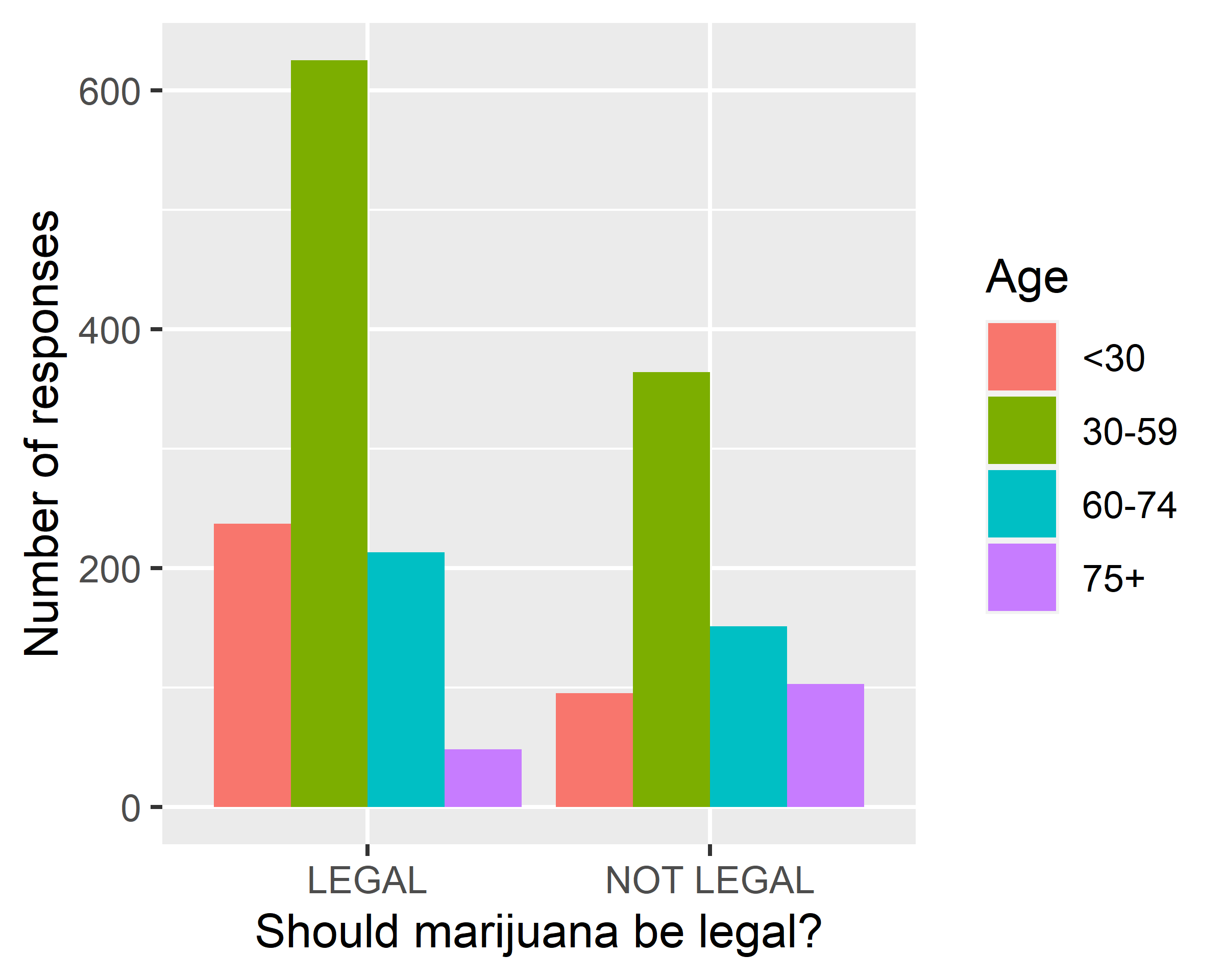
#> LEGAL 237 625 213 48 3
#> NOT LEGAL 95 364 151 103 4
#> <NA> 149 528 234 110 3
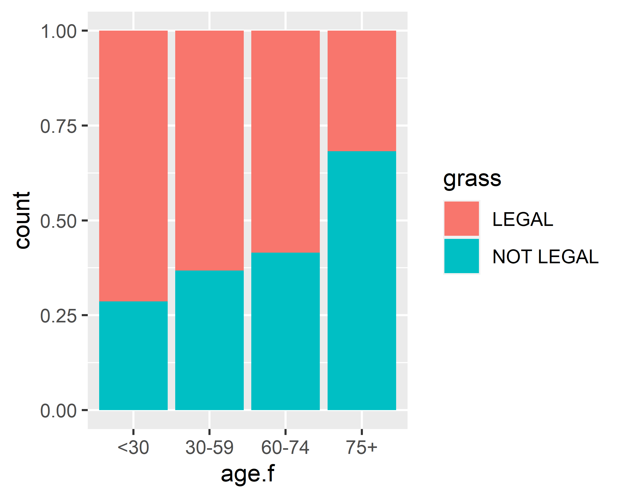
Desc(grass~age.f, data=gss.2016, plot=F)
#> ---------------------------------------------------------------
#> grass ~ age.f (gss.2016)
#>
#> Summary:
#> n: 1'836, rows: 2, columns: 4
#>
#> Pearson's Chi-squared test:
#> X-squared = 72.253, df = 3, p-value = 1.405e-15
#> Log likelihood ratio (G-test) test of independence:
#> G = 71.218, X-squared df = 3, p-value = 2.331e-15
#> Mantel-Haenszel Chi-squared:
#> X-squared = 59.423, df = 1, p-value = 1.271e-14
#>
#> Phi-Coefficient 0.198
#> Contingency Coeff. 0.195
#> Cramer's V 0.198
#>
#>
#> age.f <30 30-59 60-74 75+ Sum
#> grass
#>
#> LEGAL freq 237 625 213 48 1'123
#> perc 12.9% 34.0% 11.6% 2.6% 61.2%
#> p.row 21.1% 55.7% 19.0% 4.3% .
#> p.col 71.4% 63.2% 58.5% 31.8% .
#>
#> NOT LEGAL freq 95 364 151 103 713
#> perc 5.2% 19.8% 8.2% 5.6% 38.8%
#> p.row 13.3% 51.1% 21.2% 14.4% .
#> p.col 28.6% 36.8% 41.5% 68.2% .
#>
#> Sum freq 332 989 364 151 1'836
#> perc 18.1% 53.9% 19.8% 8.2% 100.0%
#> p.row . . . . .
#> p.col . . . . .
#> 3.5 Plots
In statistics and other sciences, being able to plot your results in the form of a graphic is often useful. An effective and accurate visualization can make your data come to life and convey your message in a powerful way. R has very powerful graphics capabilities that can help you visualize your data. In this chapter, we give you a look at traditional graphics and ggplot2 graphics.
We will look at five methods of visualizing data:
- Scatterplot
- Bar plot
- Box plot
- Histogram
- One-dimensional strip plot
3.5.1 Traditional graphics
With traditional graphics, you can create many different types of plots, such as scatterplots and bar charts. Here are just a few of the different types of plots you can create:
- Scatterplot:
plot(),stripchart() - Bar plot:
barplot() - Box plot:
boxplot() - Histogram:
hist() - One-dimensional strip plot:
stripchart()
For a complete list of the different types of plots, see the Help at
?graphics.
3.5.1.1 Bar plot
A bar plot displays the distribution (frequency) of a categorical variable through vertical or horizontal bars. In its simplest form, the format of the barplot() function is
par(mar = c(2, 2, 2, 0.1), las=1, mgp=c(2.5,0.1, 0), tcl=0.15)
barplot(table(gss.2016$age.f))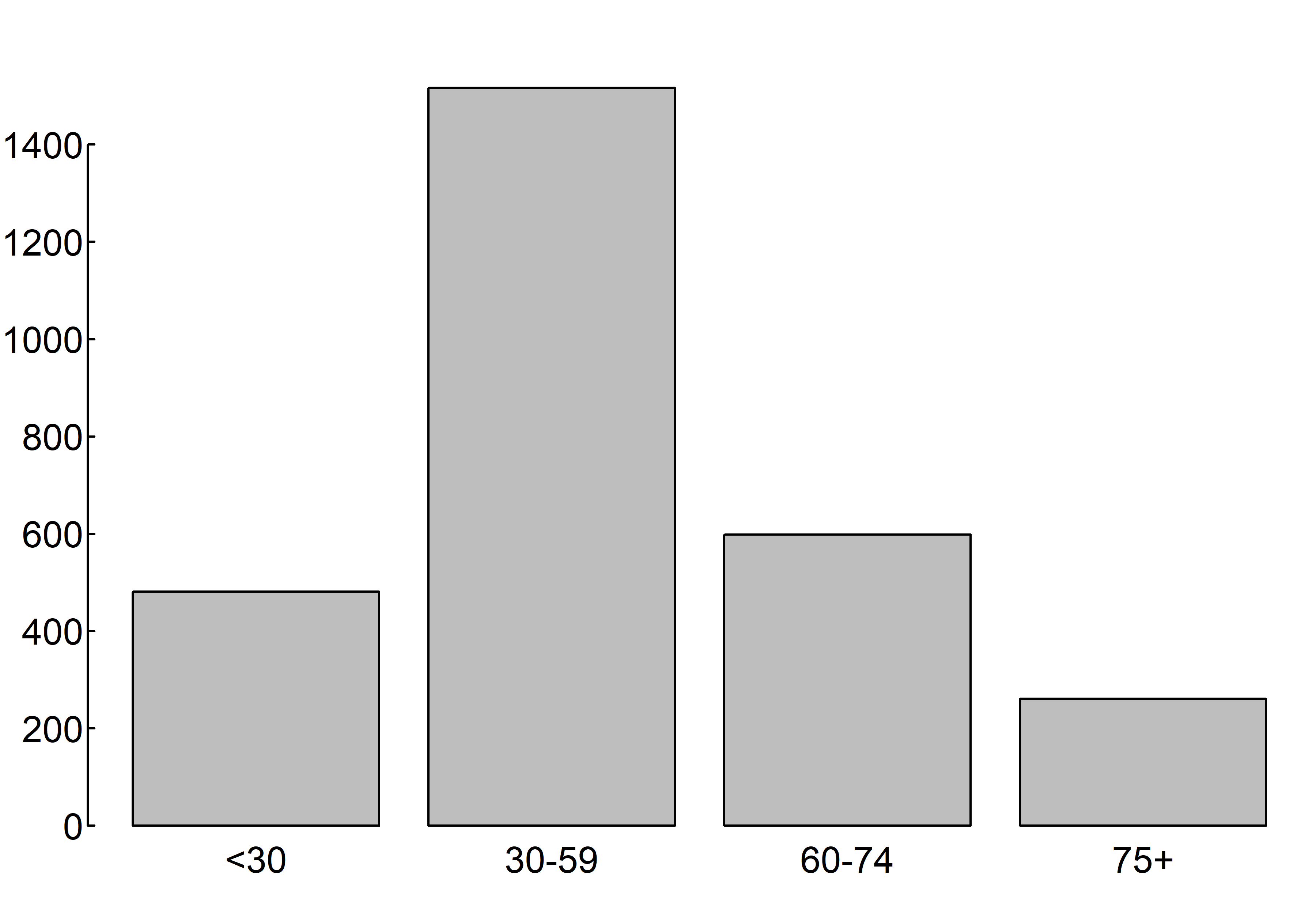
where gss.2016$age.f is a factor.
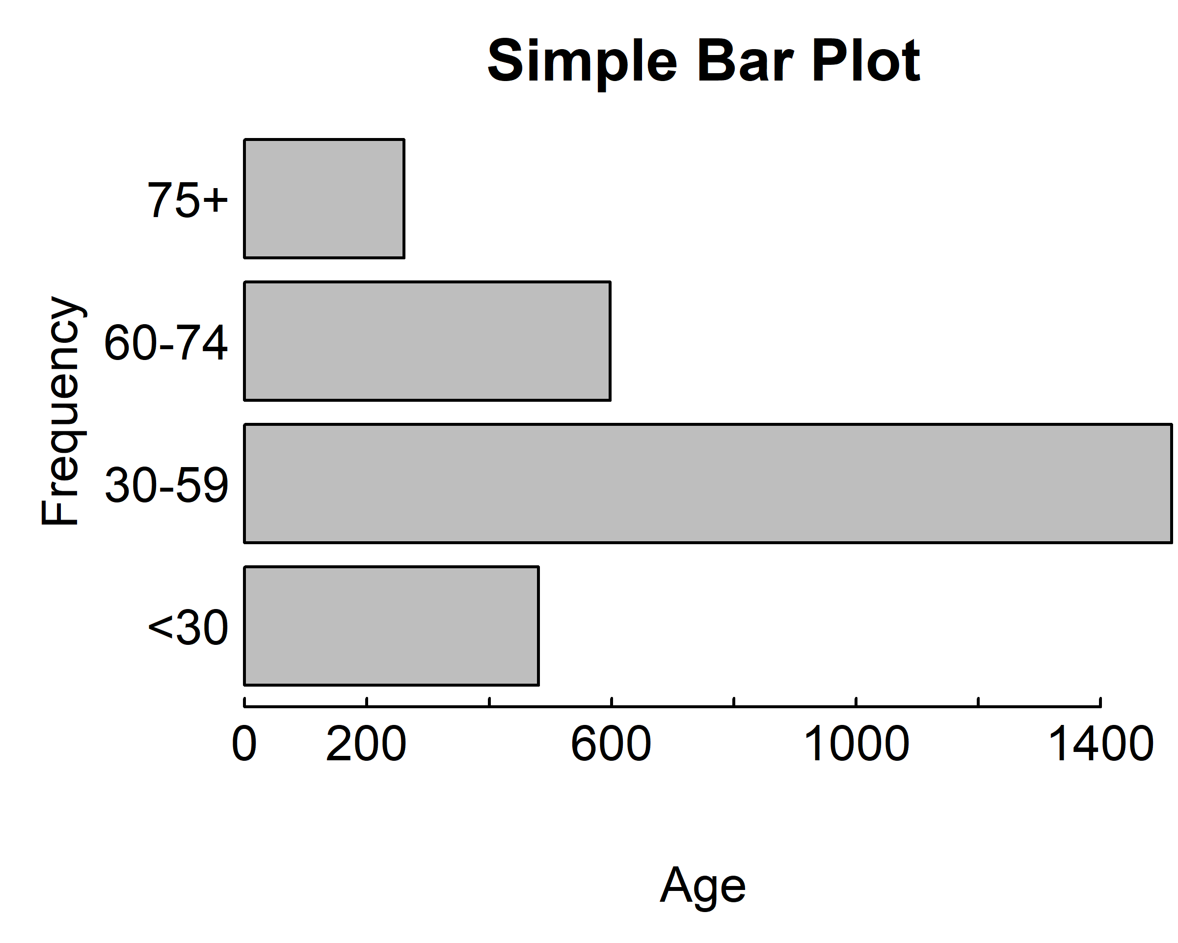
The values table(gss.2016$age.f) determine the heights of the bars in the plot, and a vertical bar plot is produced. Including the option horiz=TRUE produces a horizontal bar chart instead. You can also add annotating options. The main option adds a plot title, whereas the xlab and ylab options add x-axis and y-axis labels, respectively.
par(mar = c(4, 4, 2, 0.1), las=1, mgp=c(2.5,0.1, 0), tcl=0.15)
counts <- table(gss.2016$age.f)
barplot(counts,
        main="Simple Bar Plot",
        xlab="Age", ylab="Frequency")
barplot(counts,
        main="Simple Bar Plot",
        xlab="Age", ylab="Frequency",
        horiz=T)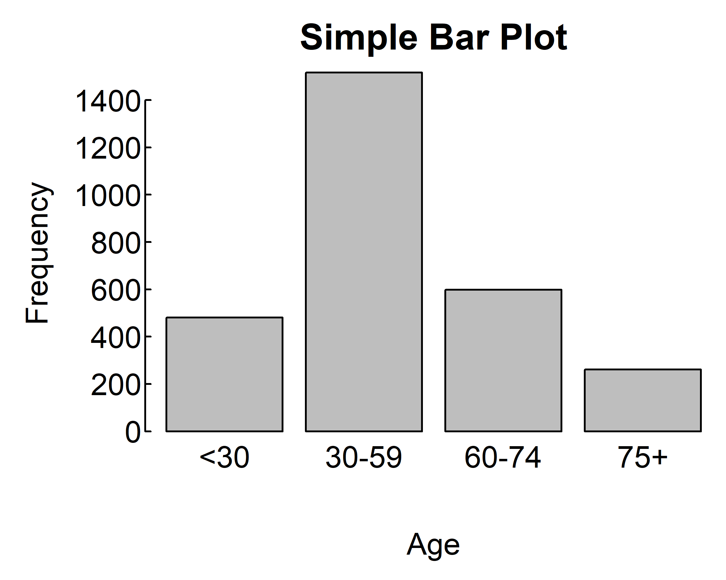
You can customize many features of a graph (fonts, colors, axes, and labels) through options called graphical parameters. One way is to specify these options through the par() function. Values set in this manner will be in effect for the rest of the session or until they’re changed. The format is par(optionname=value, optionname=value, ...). Specifying par() without parameters produces a list of the current graphical settings.
The relevant parameters are shown below
| Parameter | Description |
|---|---|
mar |
A numerical vector of the form c(bottom, left, top, right) which gives the number of lines of margin to be specified on the four sides of the plot. The default is c(5, 4, 4, 2) + 0.1. |
las |
Specifies that labels are parallel (= 0) or perpendicular (= 2) to the axis. |
tck |
Length of each tick mark as a fraction of the plotting region (a negative number is outside the graph, a positive number is inside, 0 suppresses ticks, and 1 creates gridlines). The default is -0.01. |
mgp |
The margin line for the axis title, axis labels and axis line. Note that mgp[1] affects title whereas mgp[2:3] affect axis. The default is c(3, 1, 0). |
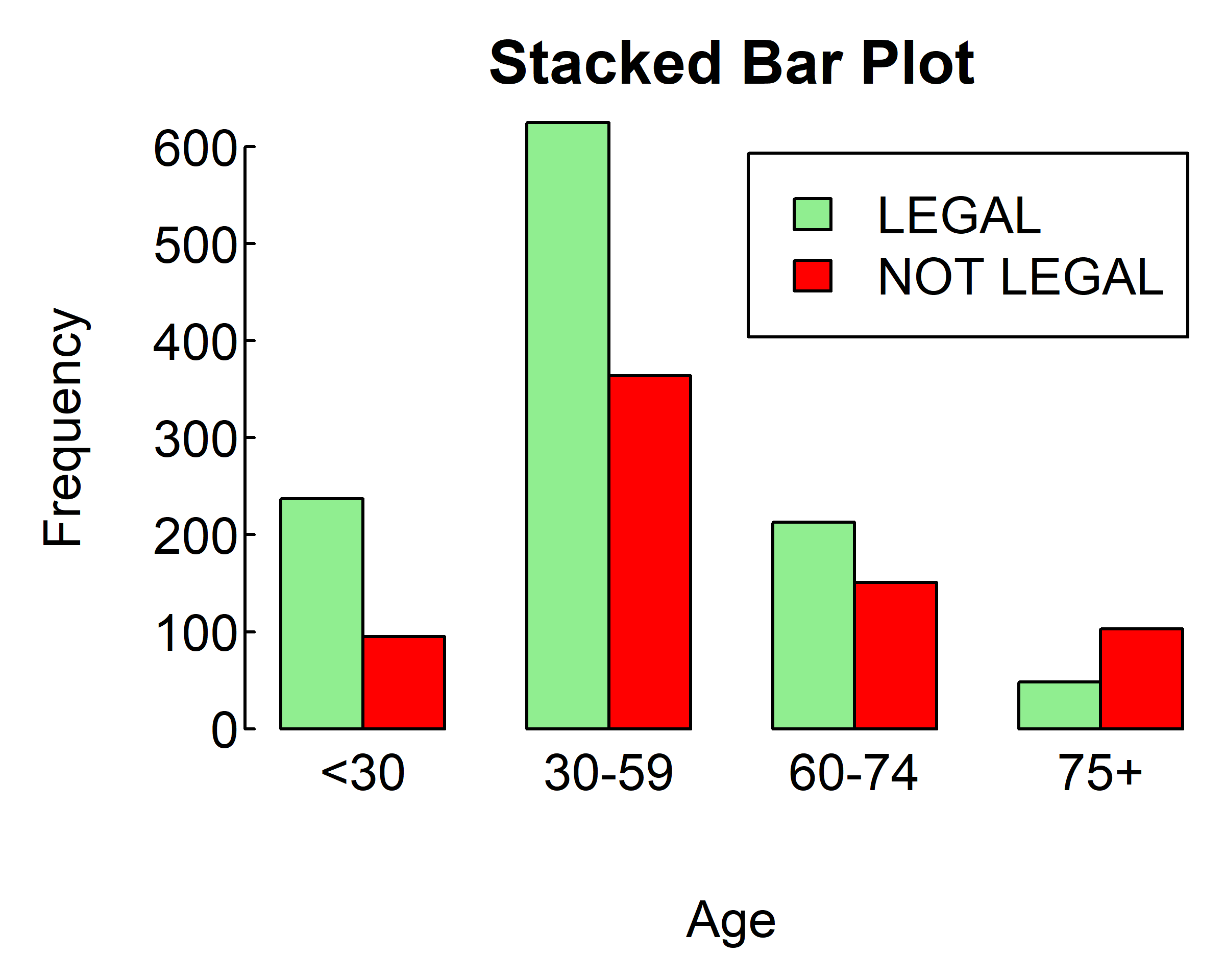
If the argument of barplot() is a matrix rather than a vector, the resulting graph will be a stacked or grouped bar plot. If beside=FALSE (the default), then each column of the matrix produces a bar in the plot, with the values in the column giving the heights of stacked “sub-bars.” If beside=TRUE, each column of the matrix represents a group, and the values in each column are juxtaposed rather than stacked.
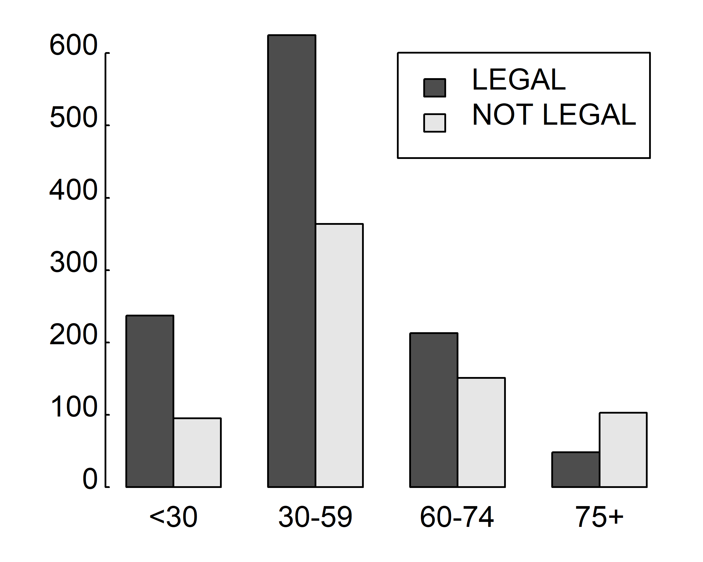
Consider the cross-tabulation of age and votes:
counts <- table(gss.2016$grass, gss.2016$age.f)
counts
#>
#>             <30 30-59 60-74 75+
#>   LEGAL     237   625   213  48
#>   NOT LEGAL  95   364   151 103
You can graph the results as either a stacked or a grouped bar plot. The resulting graphs are displayed below
par(mar = c(4, 4, 2, 0.1), las=1, mgp=c(2.5,0.1, 0), tcl=0.15)
barplot(counts,
        main="Stacked Bar Plot",
        xlab="Age", ylab="Frequency",
        col=c("lightgreen", "red"),
        legend=T)
barplot(counts,
        main="Stacked Bar Plot",
        xlab="Age", ylab="Frequency",
        col=c("lightgreen", "red"),
        legend=T, beside = T)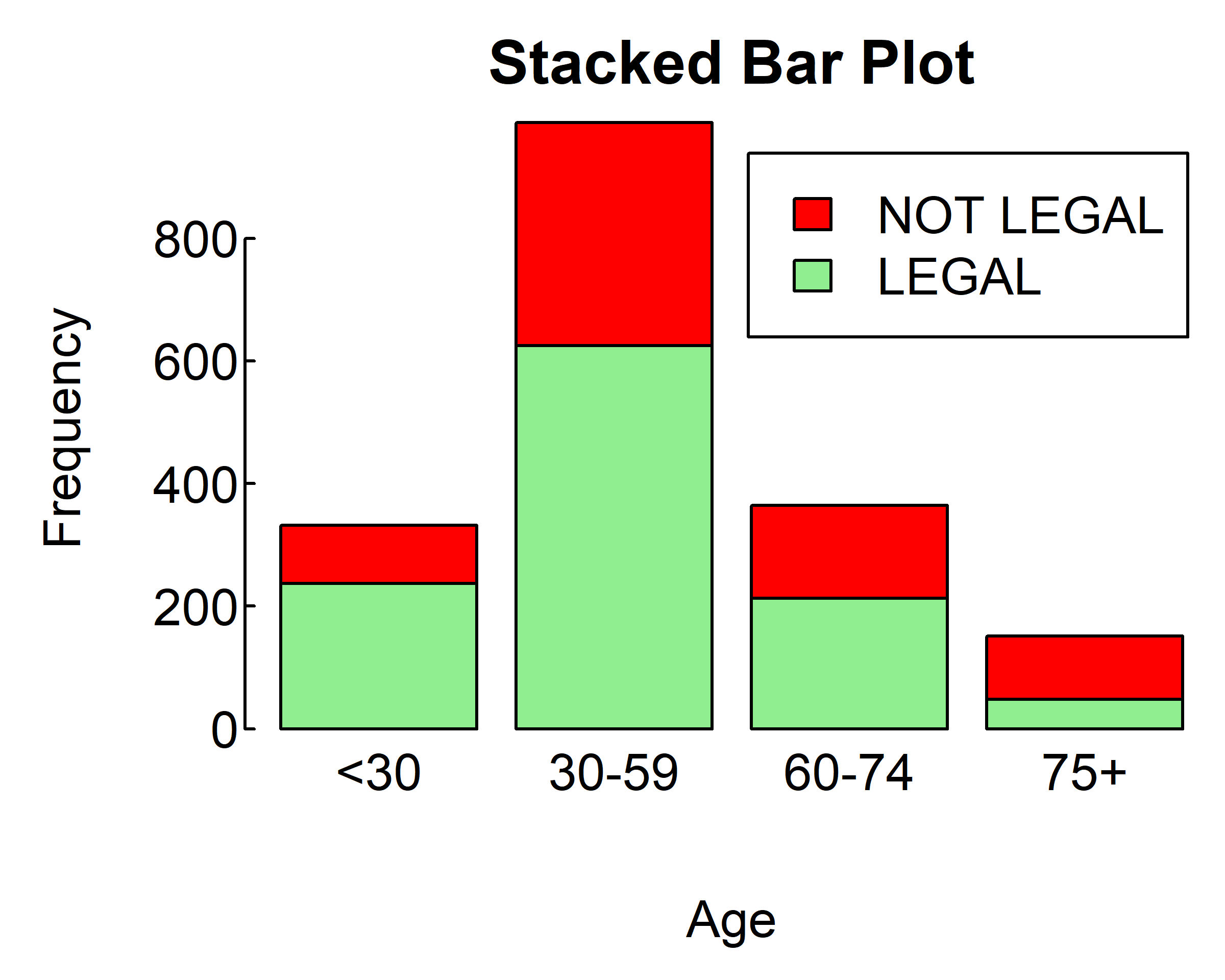
Bar plots needn’t be based on counts or frequencies. You can create bar plots that represent means, medians, standard deviations, and so forth by using the aggregate function and passing the results to the barplot() function. The following listing shows an example, which is displayed below.
par(mar = c(4, 4, 2, 0.1), las=1, mgp=c(2.5,0.1, 0), tcl=0.15)
means <- aggregate(survey$Height,
                   survey[,"Sex",drop=F], mean, na.rm=T)
means
#>      Sex        x
#> 1 Female 165.6867
#> 2   Male 178.8260
barplot(means$x, names.arg = means$Sex,
        main="Mean height")
barplot(means$x, names.arg = means$Sex,
        main="Mean height", horiz = T)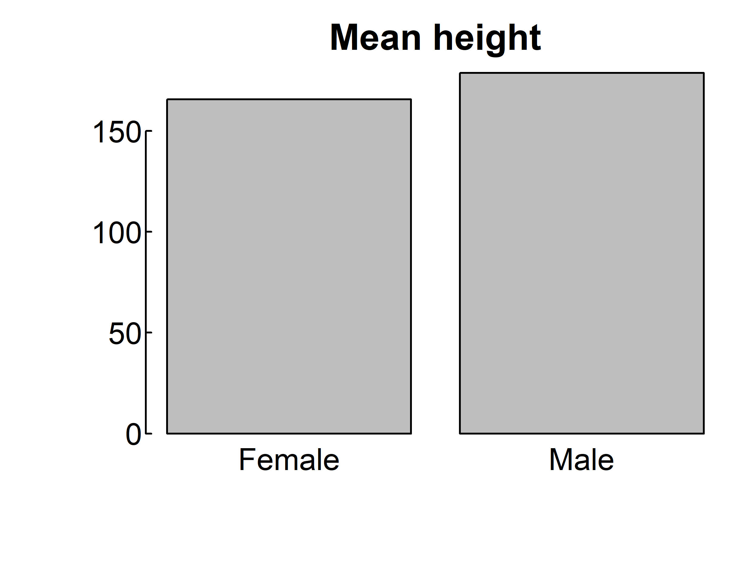
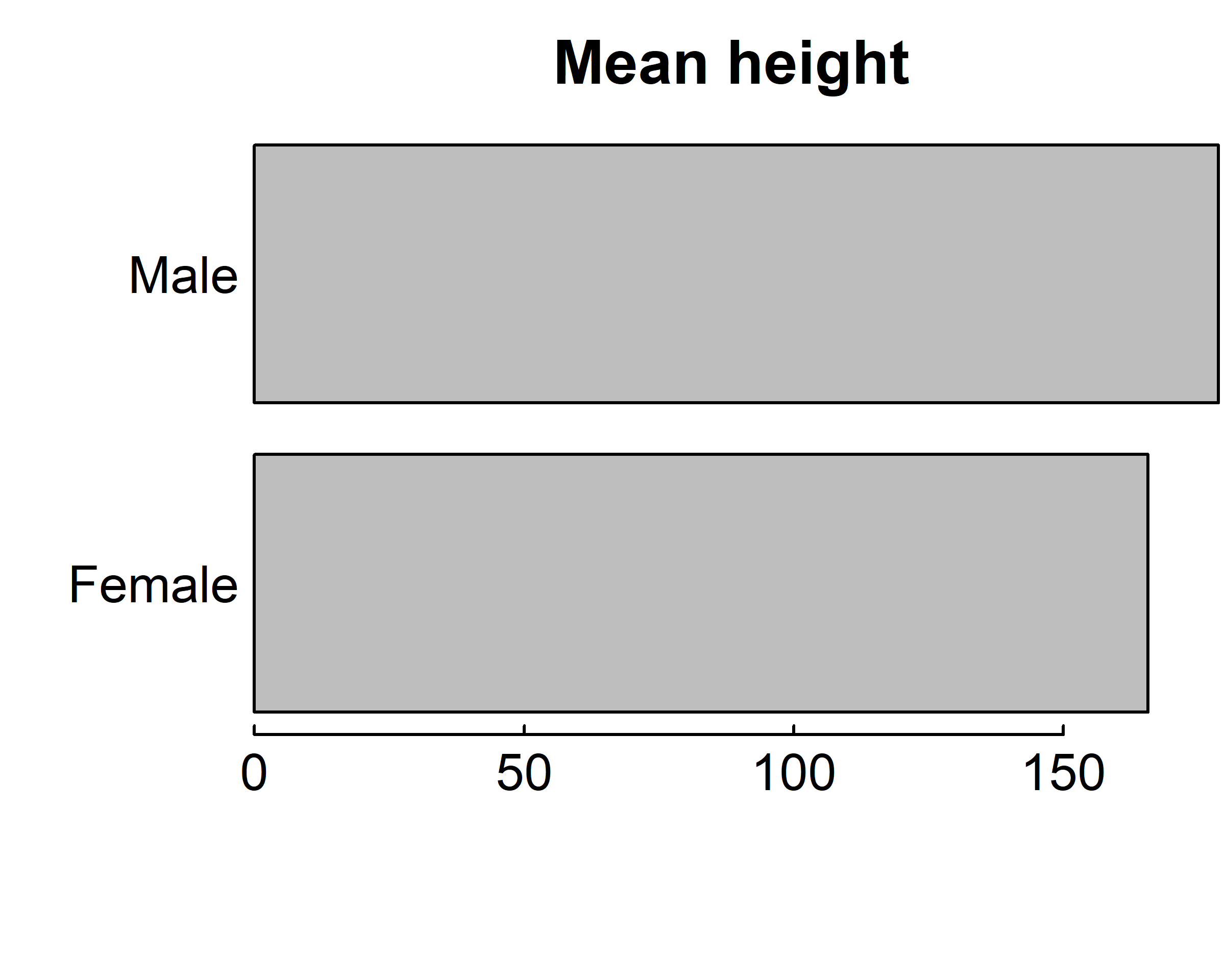
means$x is the vector containing the heights of the bars, and the option names.arg=means$Sex is added to provide labels.
Please study carefully the following codes and outputs:
par(mar = c(4, 4, 2, 0.1), las=1, mgp=c(2.5,0.1, 0), tcl=0.15)
barplot(table(gss.2016$age.f))
barplot(table(gss.2016$grass))
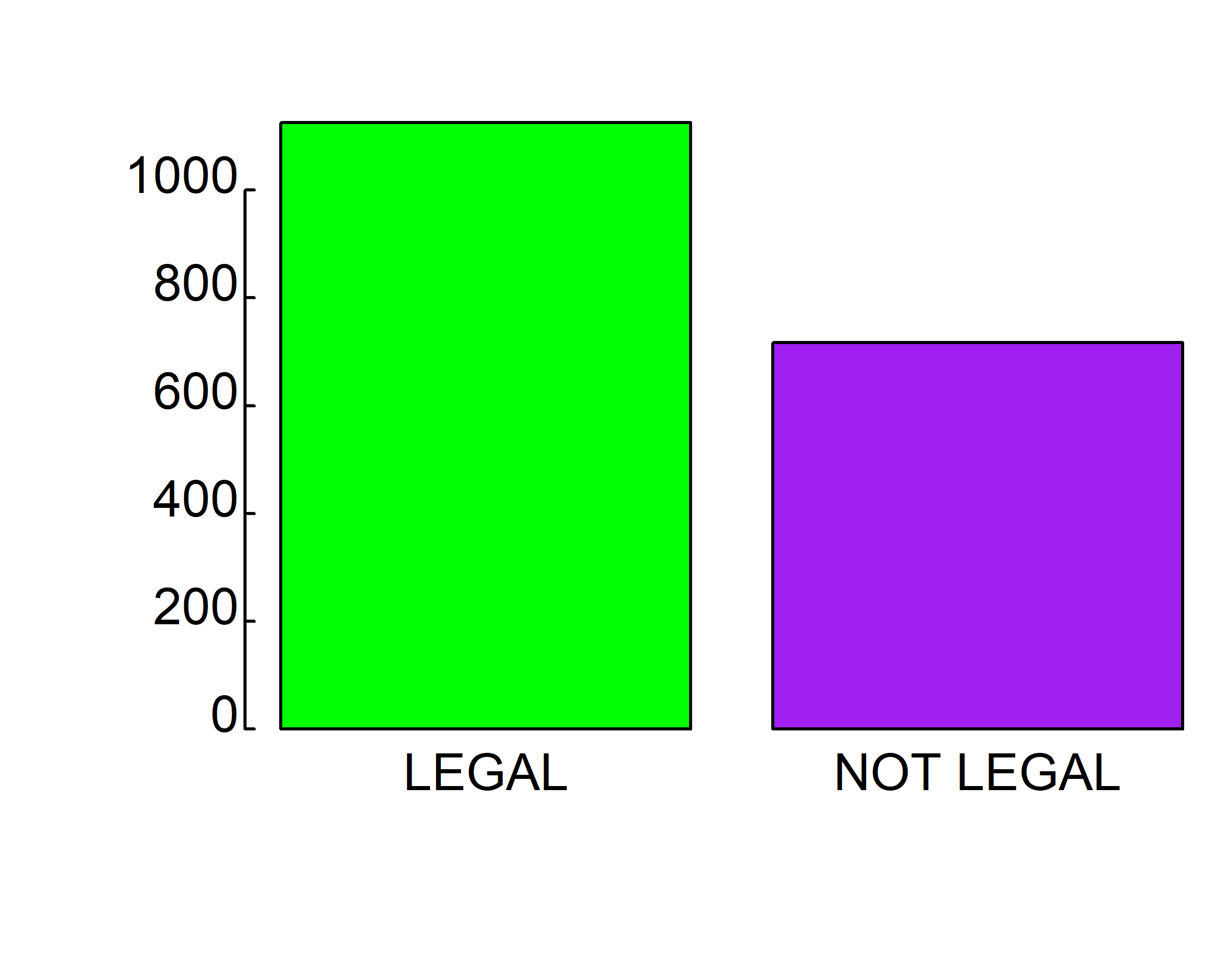
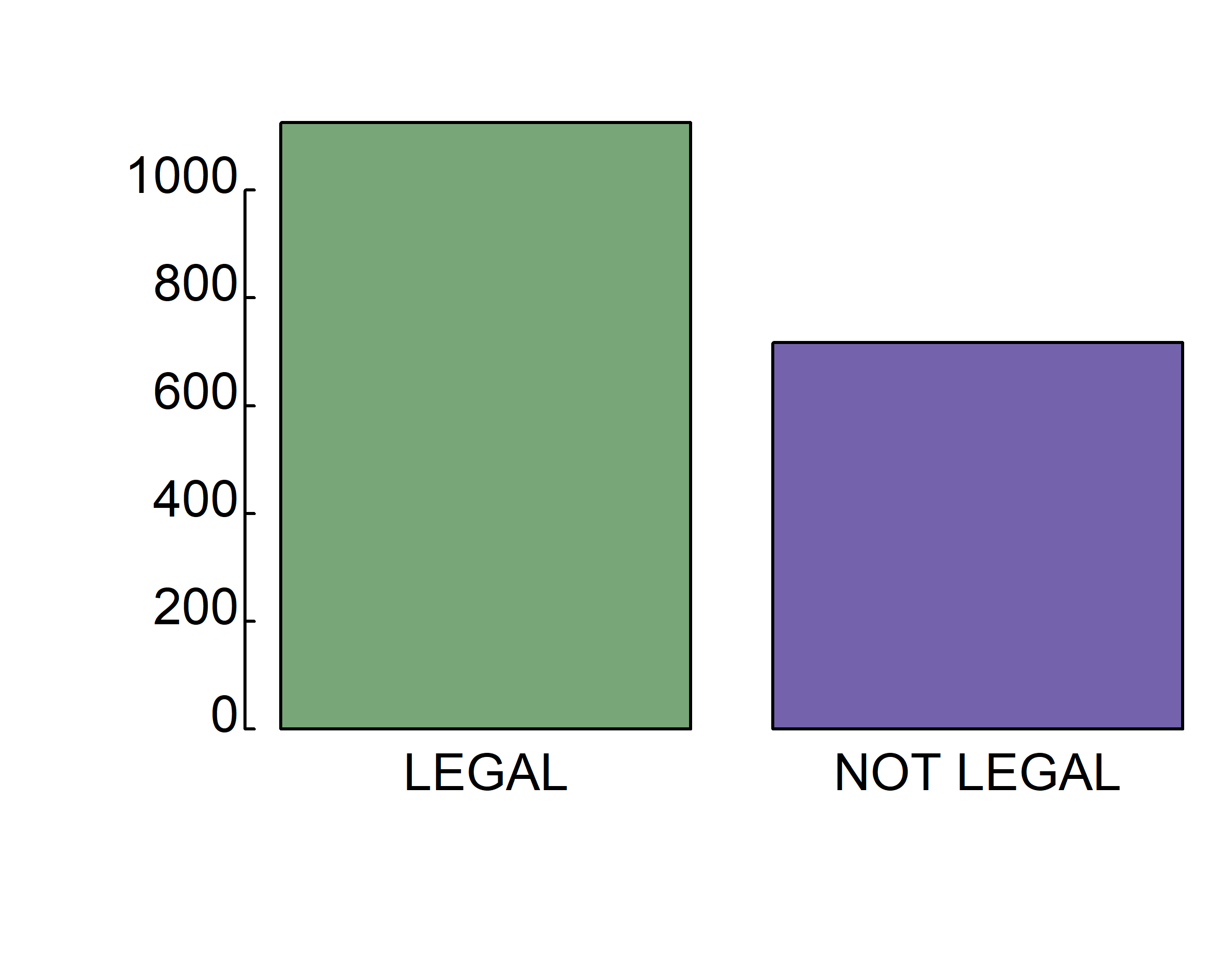
barplot(table(gss.2016$grass), col=c("green", "purple"))
barplot(table(gss.2016$grass), col=c("#78A678", "#7463AC"))
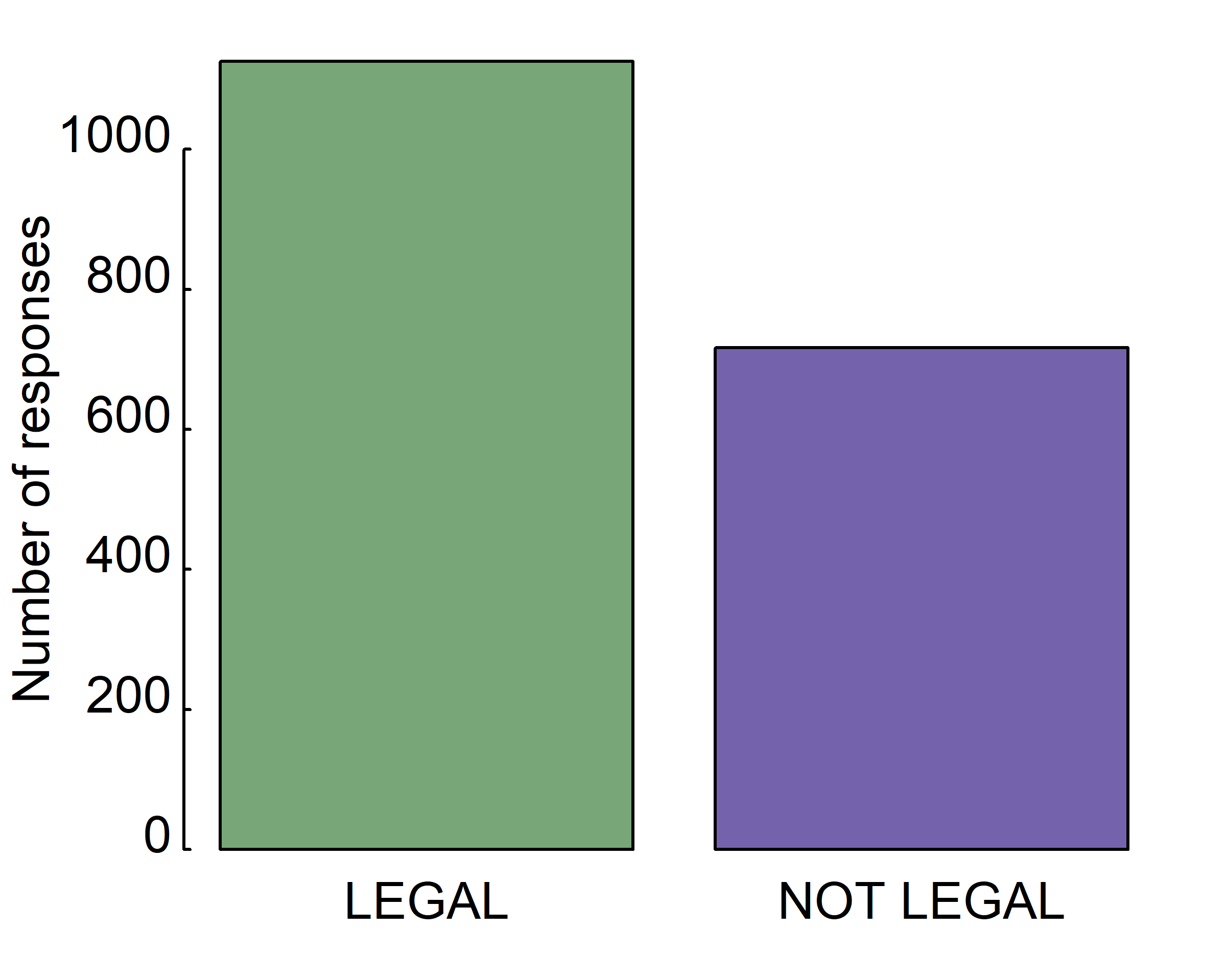
barplot(table(gss.2016$grass), col=c("#78A678", "#7463AC"),
xlab="Should marijuana be legal?", ylab="Number of responses")
par(las=1, mgp=c(2,0.2,0), tcl=0.1, mar=c(2,3,1,1))
barplot(table(gss.2016$grass), col=c("#78A678", "#7463AC"),
xlab="Should marijuana be legal?", ylab="Number of responses")
# to save plot to PNG
par(las=1, mgp=c(2,0.2,0), tcl=0.1, mar=c(2,3,1,1))
barplot(table(gss.2016$grass, gss.2016$age.f), beside = T, legend=T)
png(filename = "output/image/barplot_1.png", width = 400, height = 300)
par(las=1, mgp=c(2,0.2,0), tcl=0.1, mar=c(2,3,1,1))
barplot(table(gss.2016$grass, gss.2016$age.f), beside = T, legend=T)
dev.off()
#> png
#> 2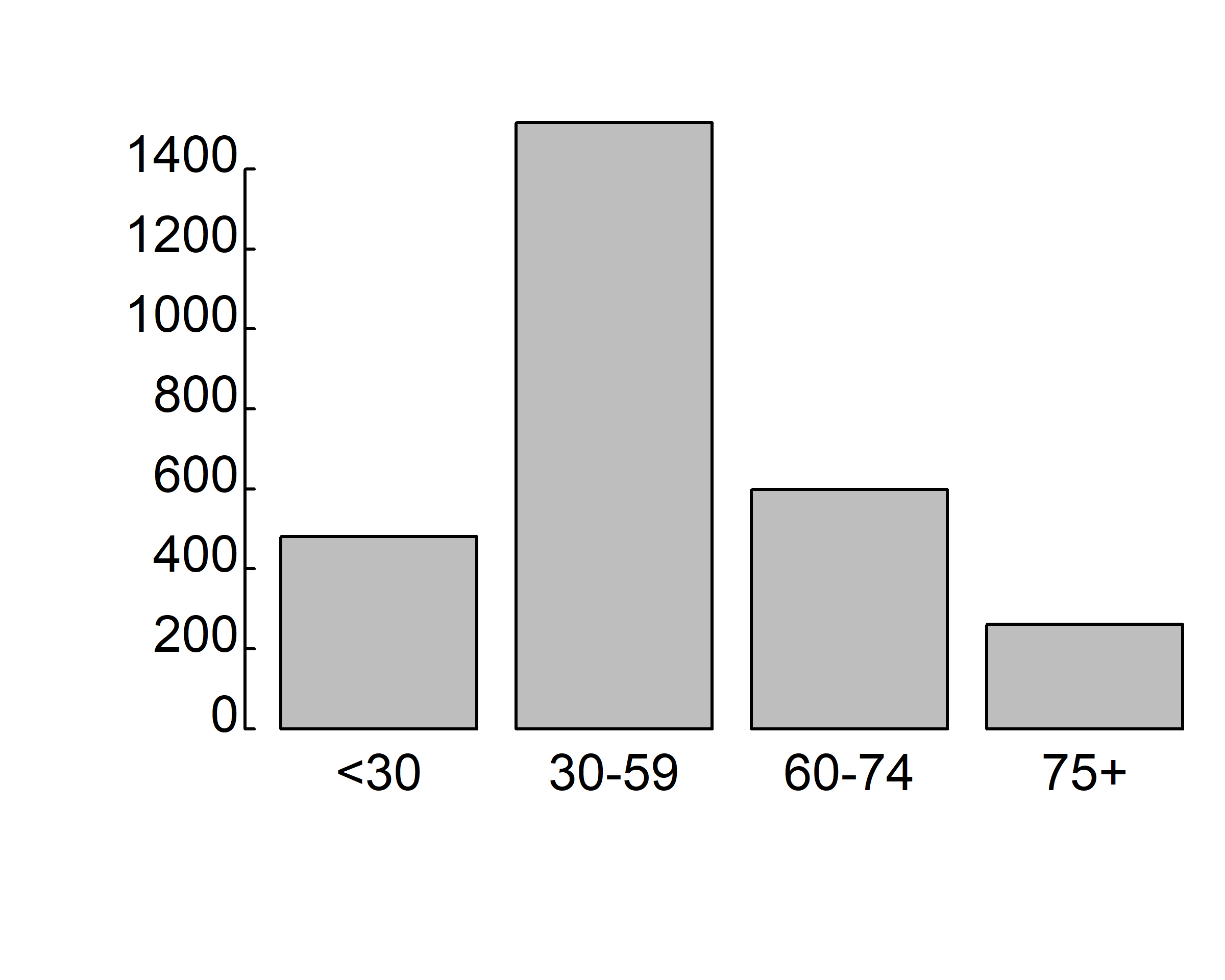
3.5.1.2 Histogram
Histograms display the distribution of a continuous variable by dividing the range of scores into a specified number of bins on the x-axis and displaying the frequency of scores in each bin on the y-axis. You can create histograms with the function
par(mar = c(2, 2, 2, 0.1), las=1, mgp=c(2.5,0.1, 0), tcl=0.15)
hist(survey$Wr.Hnd)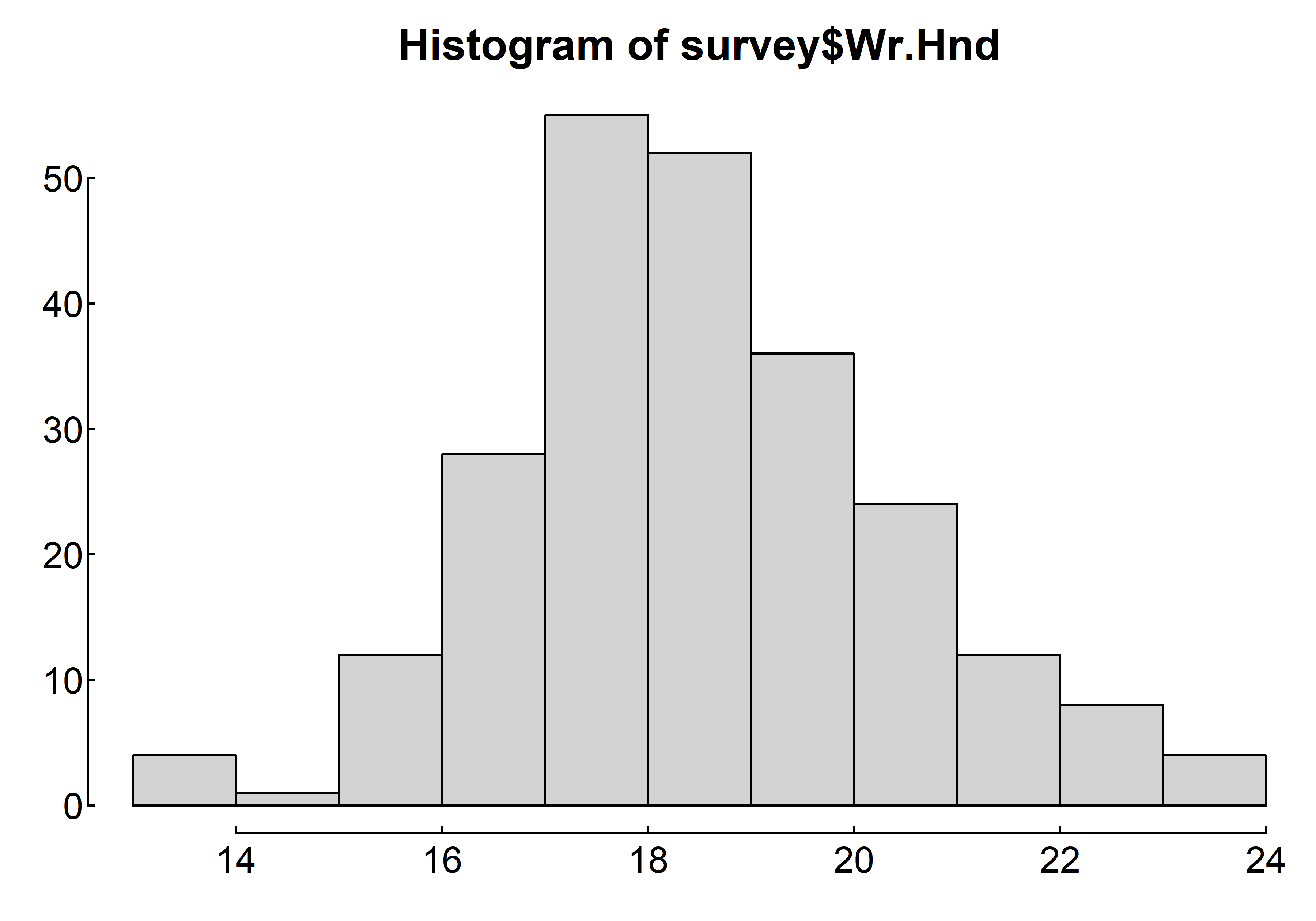
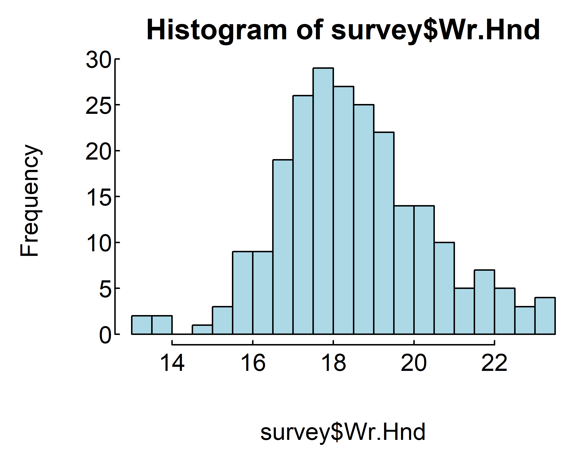
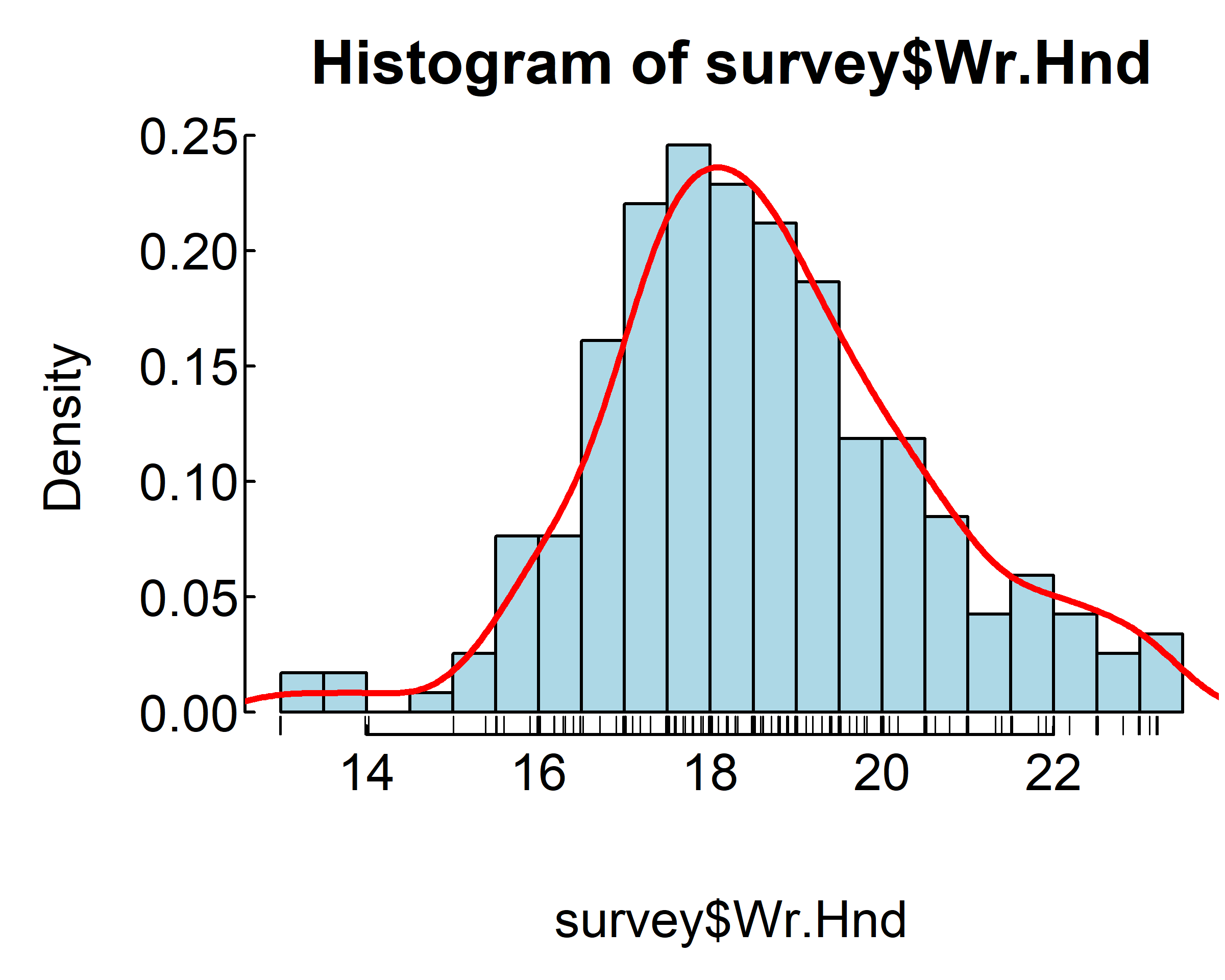
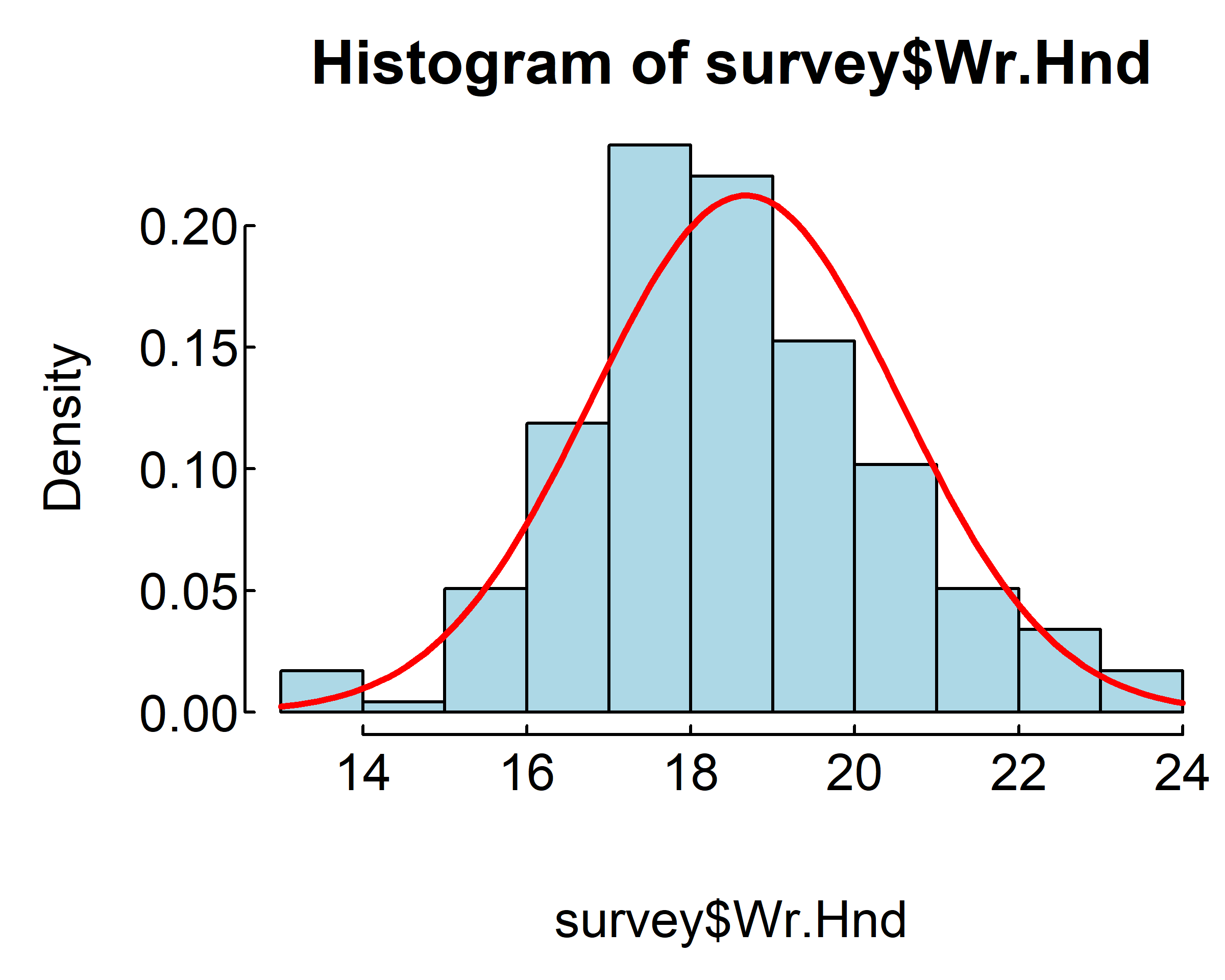
where survey$Wr.Hnd is a numeric vector of values. The option freq=FALSE creates a plot based on probability densities rather than frequencies. The breaks= option controls the number of bins. The default produces equally spaced breaks when defining the cells of the histogram. The following listing provides the code for four variations of a histogram; the results are plotted in figure 6.8.
par(mar = c(4, 4, 2, 0.1), las=1, mgp=c(2.5,0.1, 0), tcl=0.15)
hist(survey$Wr.Hnd)
hist(survey$Wr.Hnd,
     breaks=20, col = "lightblue")
hist(survey$Wr.Hnd,
     breaks=20, col = "lightblue",
     freq = F)
rug(jitter(survey$Wr.Hnd))
lines(density(survey$Wr.Hnd, na.rm = TRUE),
      col="red", lwd=2)
range(survey$Wr.Hnd, na.rm = T)
#> [1] 13.0 23.2
hist(survey$Wr.Hnd,
     breaks=seq(from=13, to=24, by=1),
     col = "lightblue", freq = F)
curve(dnorm(x, mean=mean(survey$Wr.Hnd, na.rm = T),
            sd=sd(survey$Wr.Hnd, na.rm = T)),
      from=13, to=24, add=T, col="red", lwd=2)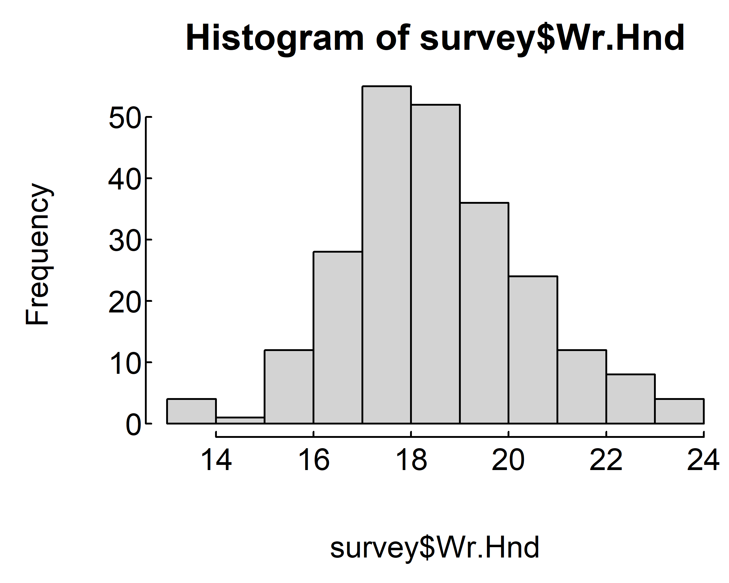
3.5.1.3 Box plot
A box-and-whiskers plot describes the distribution of a continuous variable by plotting its five-number summary: the minimum, lower quartile (25th percentile), median (50th percentile), upper quartile (75th percentile), and maximum. It can also display observations that may be outliers (values outside the range of \(\pm1.5*IQR\), where IQR is the interquartile range defined as the upper quartile minus the lower quartile). For example, this statement produces the plot shown below:
par(mar = c(2, 2, 2, 0.1), las=1, mgp=c(2.5,0.1, 0), tcl=0.15)
boxplot(survey$Wr.Hnd, main="Box plot", ylab="cm")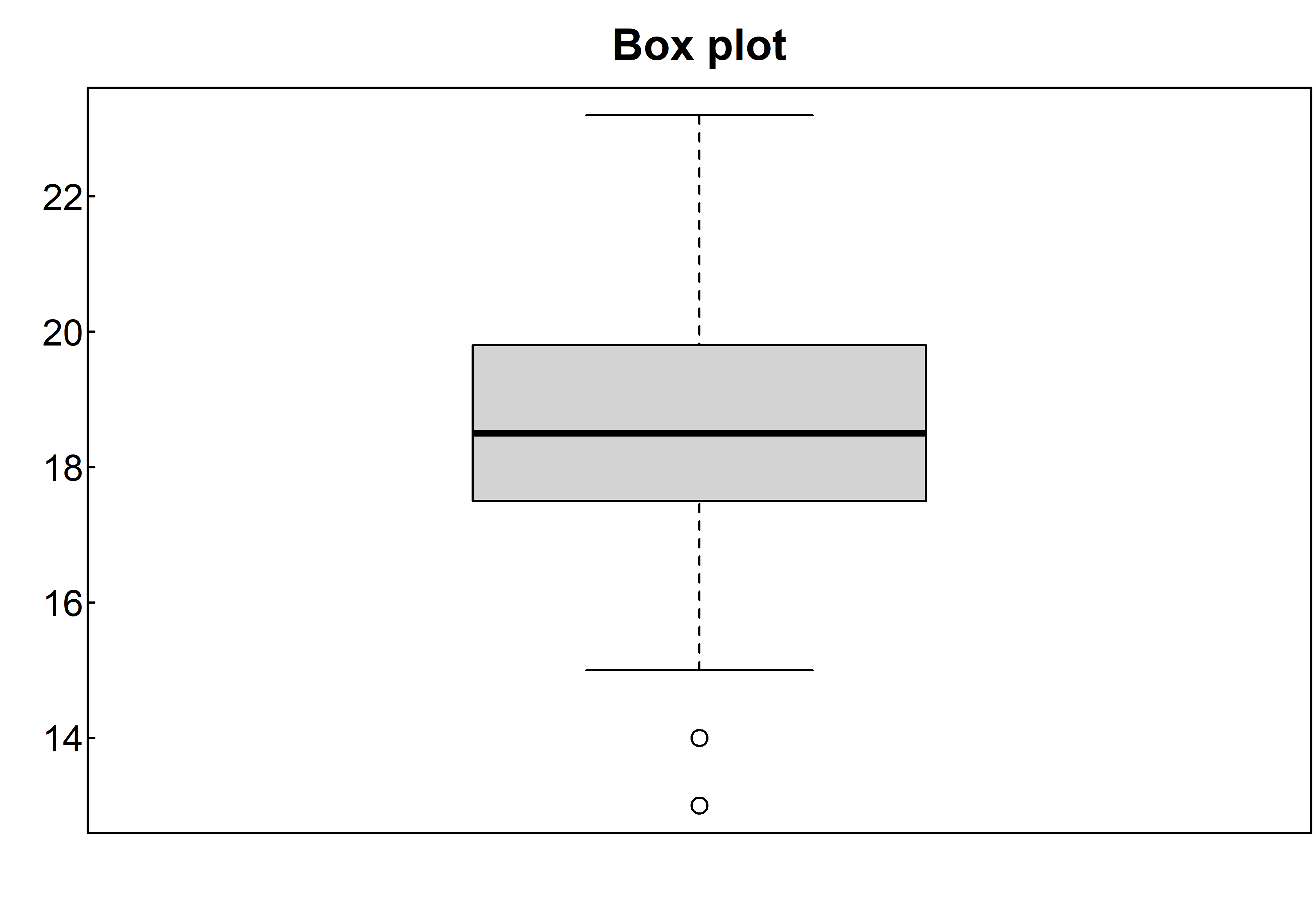
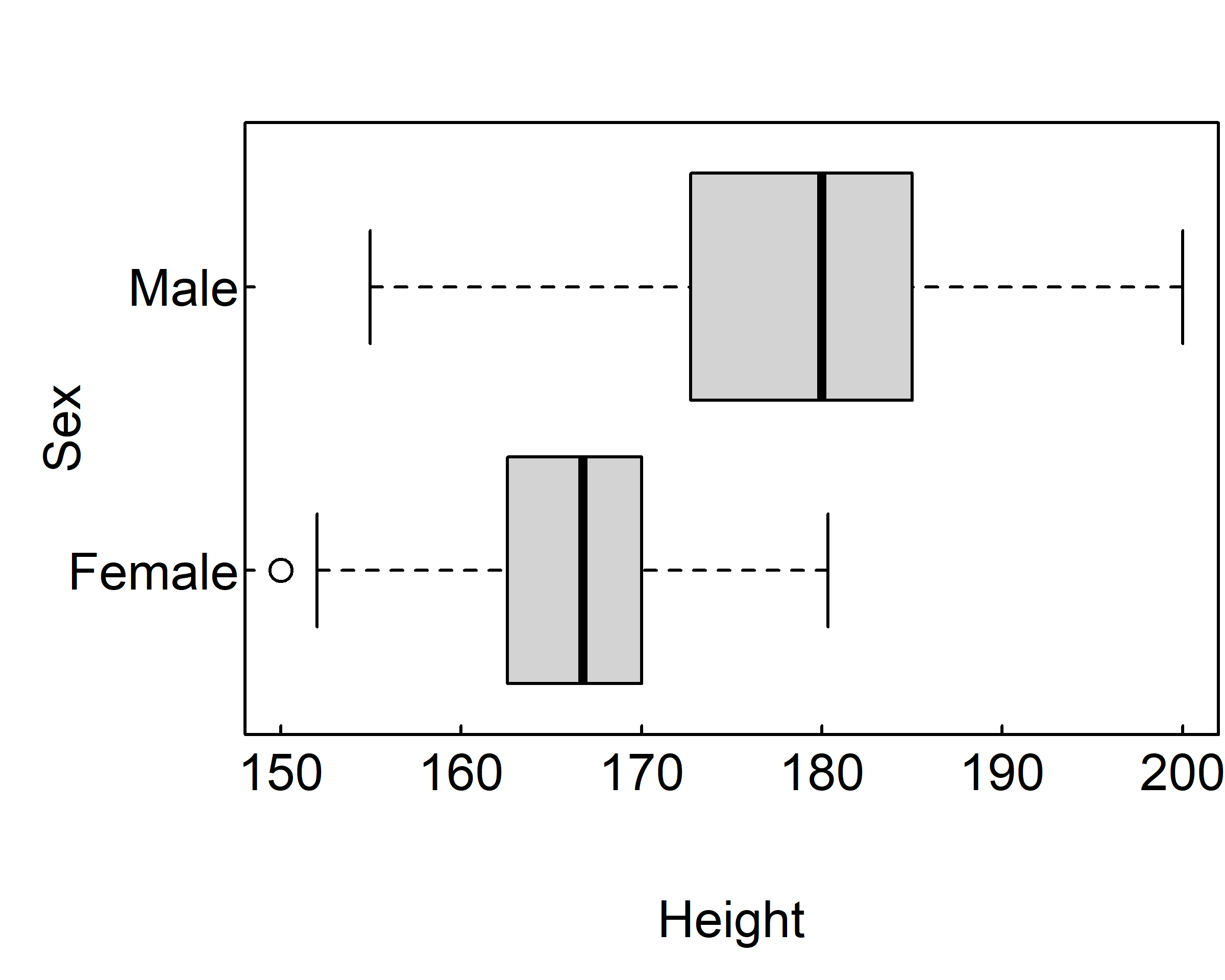
Box plots can be created for individual variables or for variables by group. The format is
boxplot(formula, data=dataframe)where formula is a formula and dataframe denotes the data frame (or list) providing the data. An example of a formula is y ~ A, where a separate box plot for numeric variable y is generated for each value of categorical variable A. The formula y ~ A*B would produce a box plot of numeric variable y, for each combination of levels in categorical variables A and B.
Adding the option horizontal=TRUE to reverse the axis orientation.
The following code revisits the impact of sex on height with parallel box plots.
par(mar = c(4, 4, 2, 0.1), las=1, mgp=c(2.5,0.1, 0), tcl=0.15)
boxplot(Height ~ Sex, data=survey)
boxplot(Height ~ Sex, data=survey, horizontal=TRUE)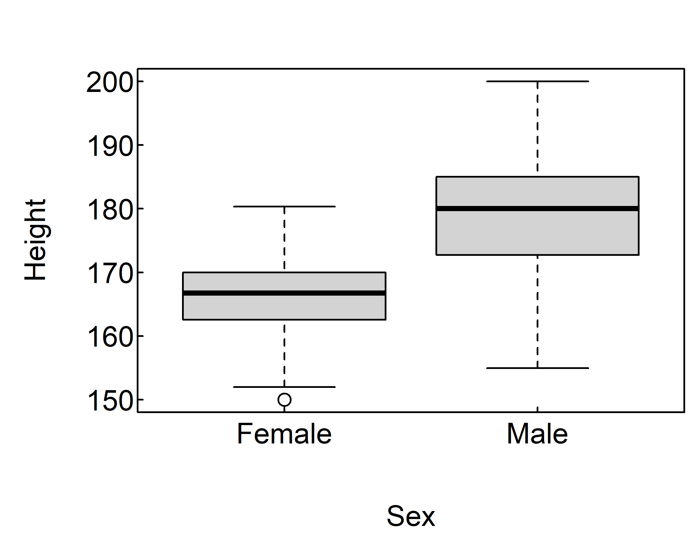
3.5.1.4 Scatterplot
To create a scatterplot, you use the plot() function. A scatterplot creates points (or sometimes bubbles or other symbols) on your chart. Each point corresponds to an observation in your data. You’ve probably seen or created this type of graphic a million times, so you already know that scatterplots use the Cartesian coordinate system, where one variable is mapped to the x‐axis and a second variable is mapped to the y‐axis.
The most common high level function used to produce plots in R is the plot() function.
par(mar = c(3, 3, 2, 0.1), las=1, mgp=c(1.5,0.1, 0), tcl=0.15)
plot(survey$Wr.Hnd)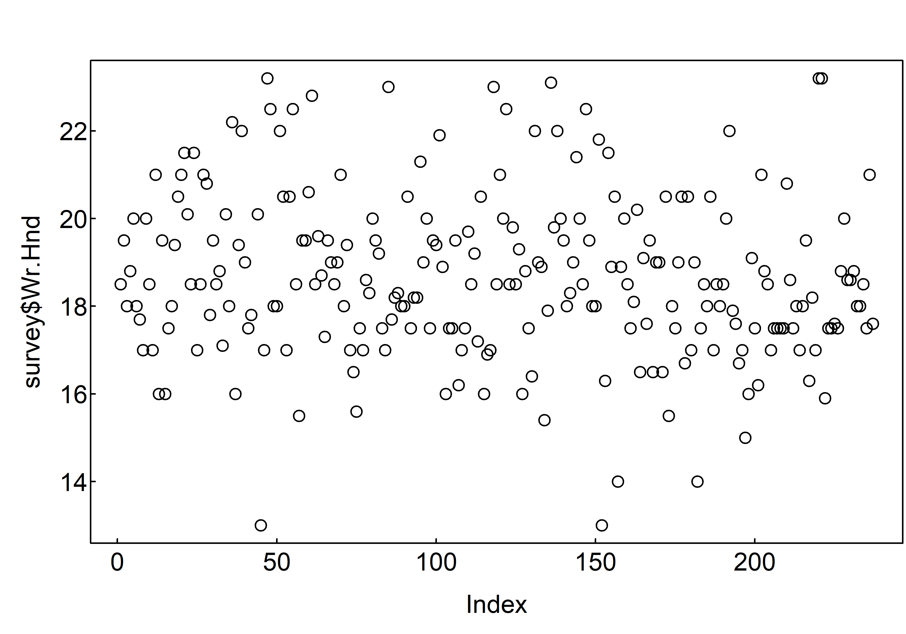
R has plotted the values of Wr.Hnd (on the y axis) against an index since we are only plotting one variable to plot. The index is just the order of the Wr.Hnd values in the data frame (1 first in the data frame and 237 last). The Wr.Hnd variable name has been automatically included as a y axis label and the axes scales have been automatically set.
To plot a scatterplot of one numeric variable against another numeric variable we just need to include both variables as arguments when using the plot() function. For example to plot Wr.Hnd on the y axis and Height of the x axis.
par(mar = c(3, 3, 2, 0.1), las=1, mgp=c(1.5,0.1, 0), tcl=0.15)
plot(x = survey$Height, y = survey$Wr.Hnd)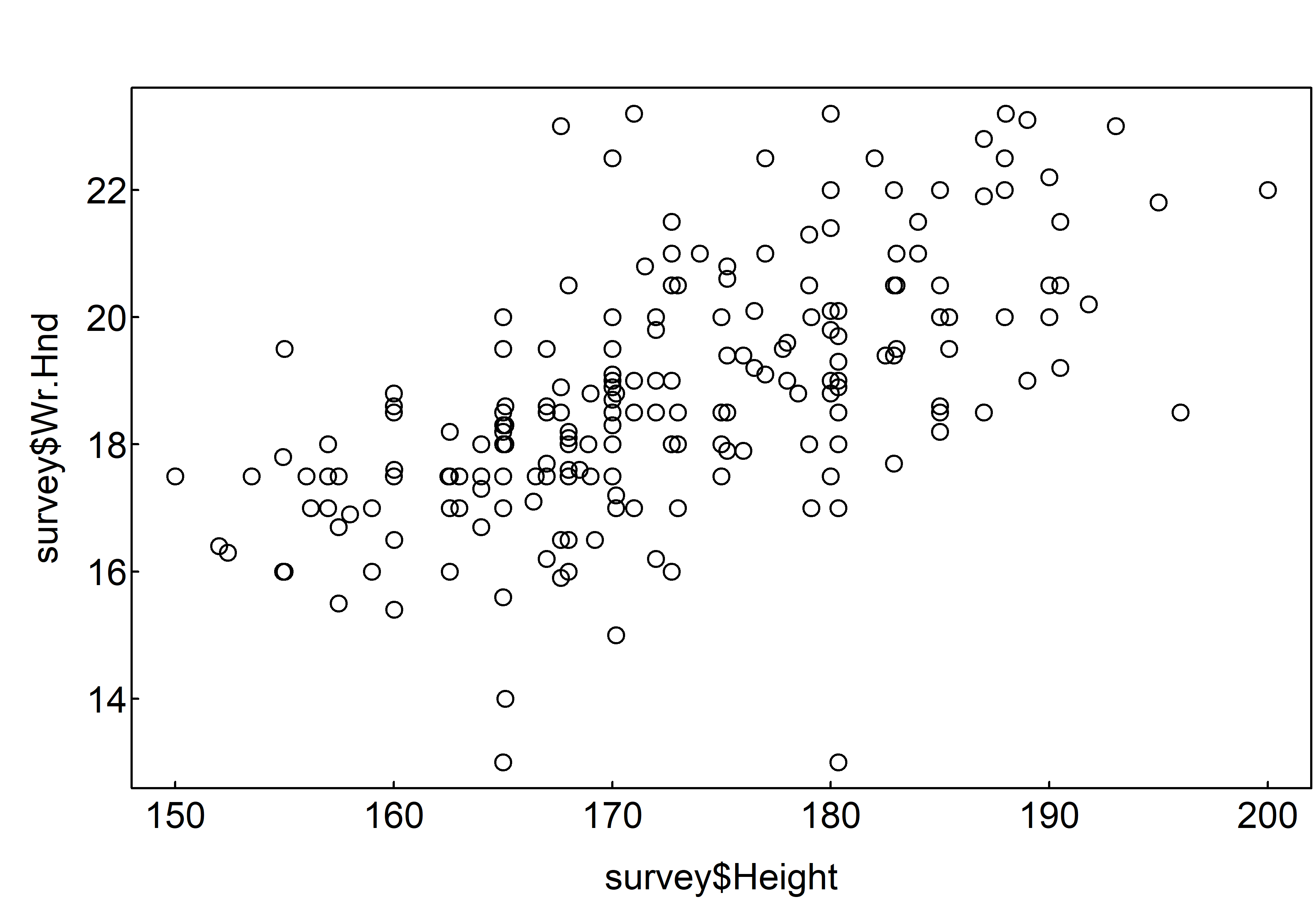
There is an equivalent approach for these types of plots which often causes some confusion at first. You can also use the formula notation when using the plot() function. However, in contrast to the previous method the formula method requires you to specify the y axis variable first, then a ~ and then our x axis variable.
par(mar = c(4, 4, 0.1, 0.1))
plot(Wr.Hnd~Height, data=survey)
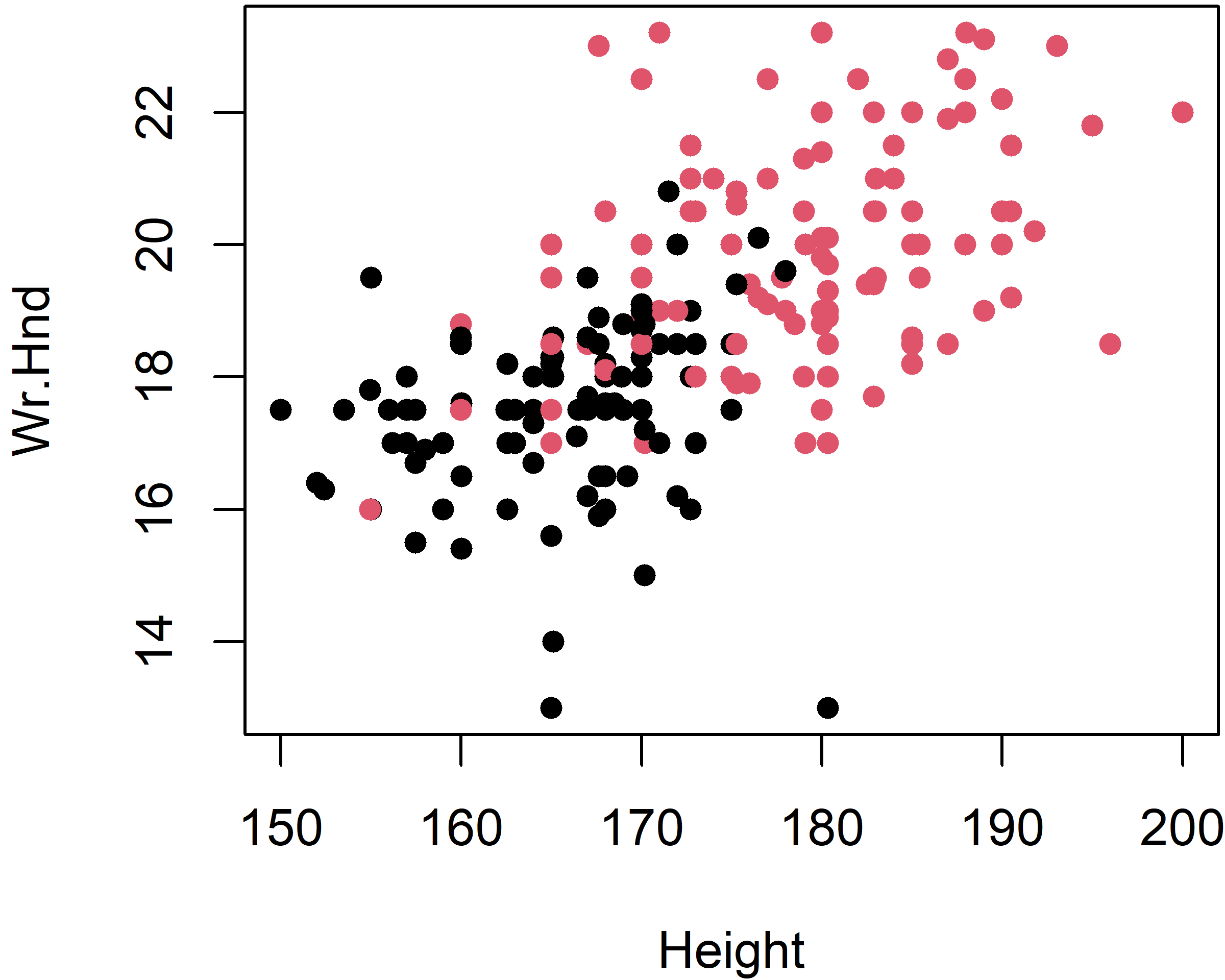
plot(Wr.Hnd~Height, data=survey, col=survey$Sex, pch=16)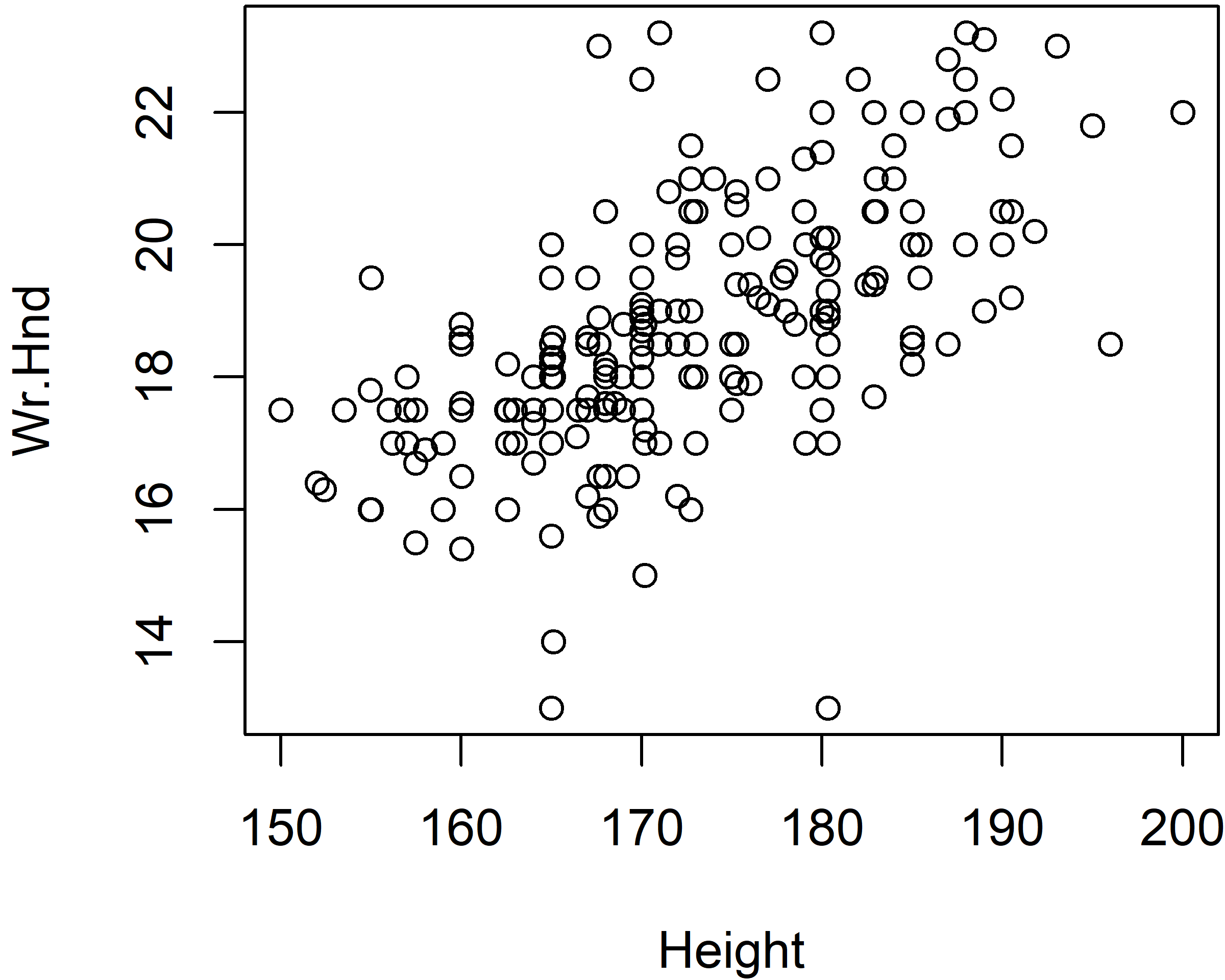
3.5.2 ggplot2 graphics
ggplot2 graphics is based on ggplot2 package. Because ggplot2 isn’t part of the standard distribution of R, you have to download the package from CRAN and install it. To install the ggplot2 package, use:
install.packages("ggplot2")And then to load the package, use:
library("ggplot2")The basic concept of a ggplot2 graphic is that you combine different plot elements into layers. Each layer of a ggplot2 graphic contains information about the following:
- The data that you want to plot: for
ggplot(), this must be a data frame. - A mapping from the data to your plot: this usually is as simple as telling
ggplot()what goes on the x‐axis and what goes on the y‐axis. - A geometric object, or geom in ggplot terminology: the geom defines the overall look of the layer (for example, whether the plot is made up of bars, points, or lines).
3.5.2.1 Bar plot
Please study carefully the following codes and outputs:
library(ggplot2)
ggplot(data = gss.2016, mapping = aes(x=age.f)) + geom_bar()
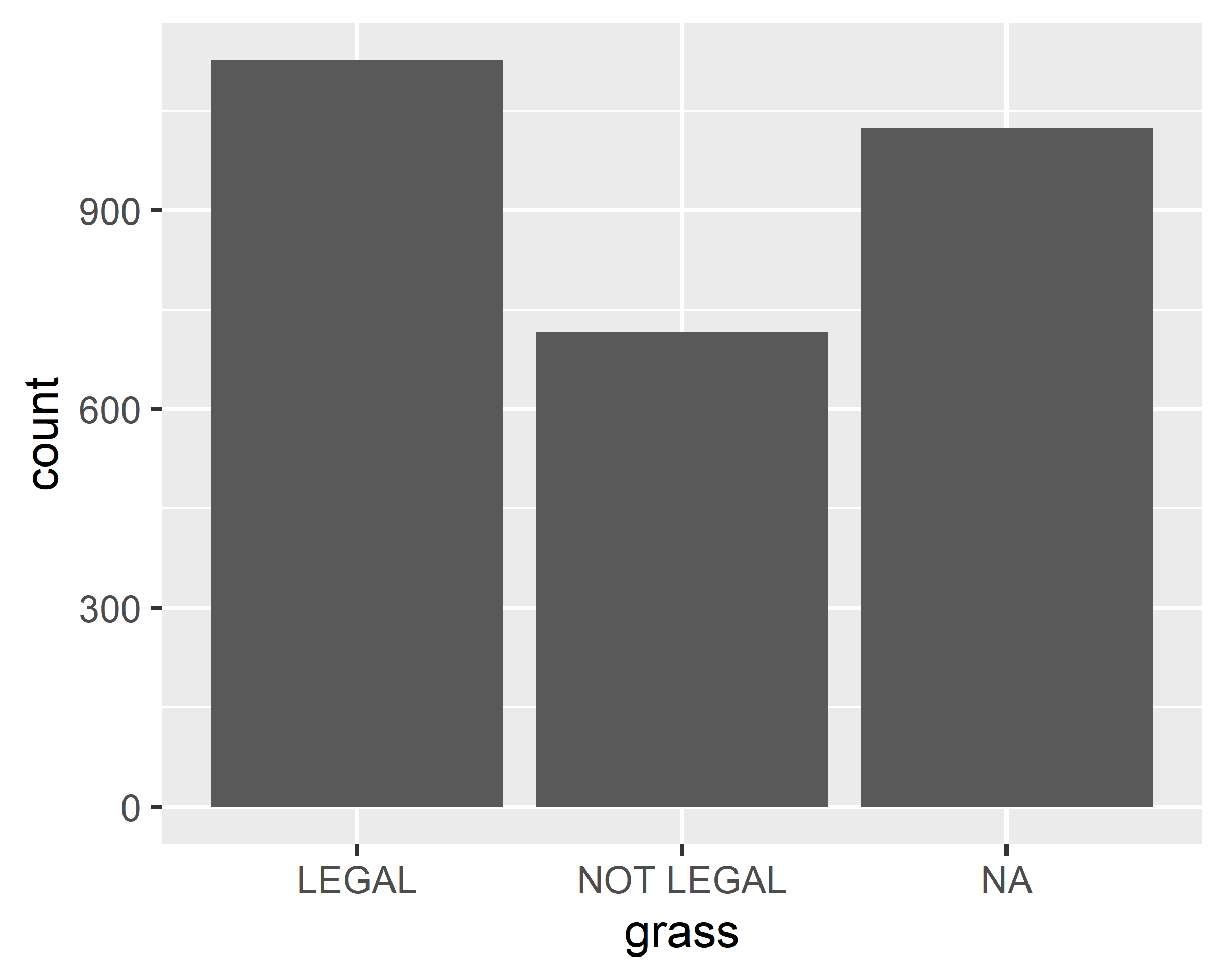
ggplot(data = gss.2016, mapping = aes(x=grass)) + geom_bar()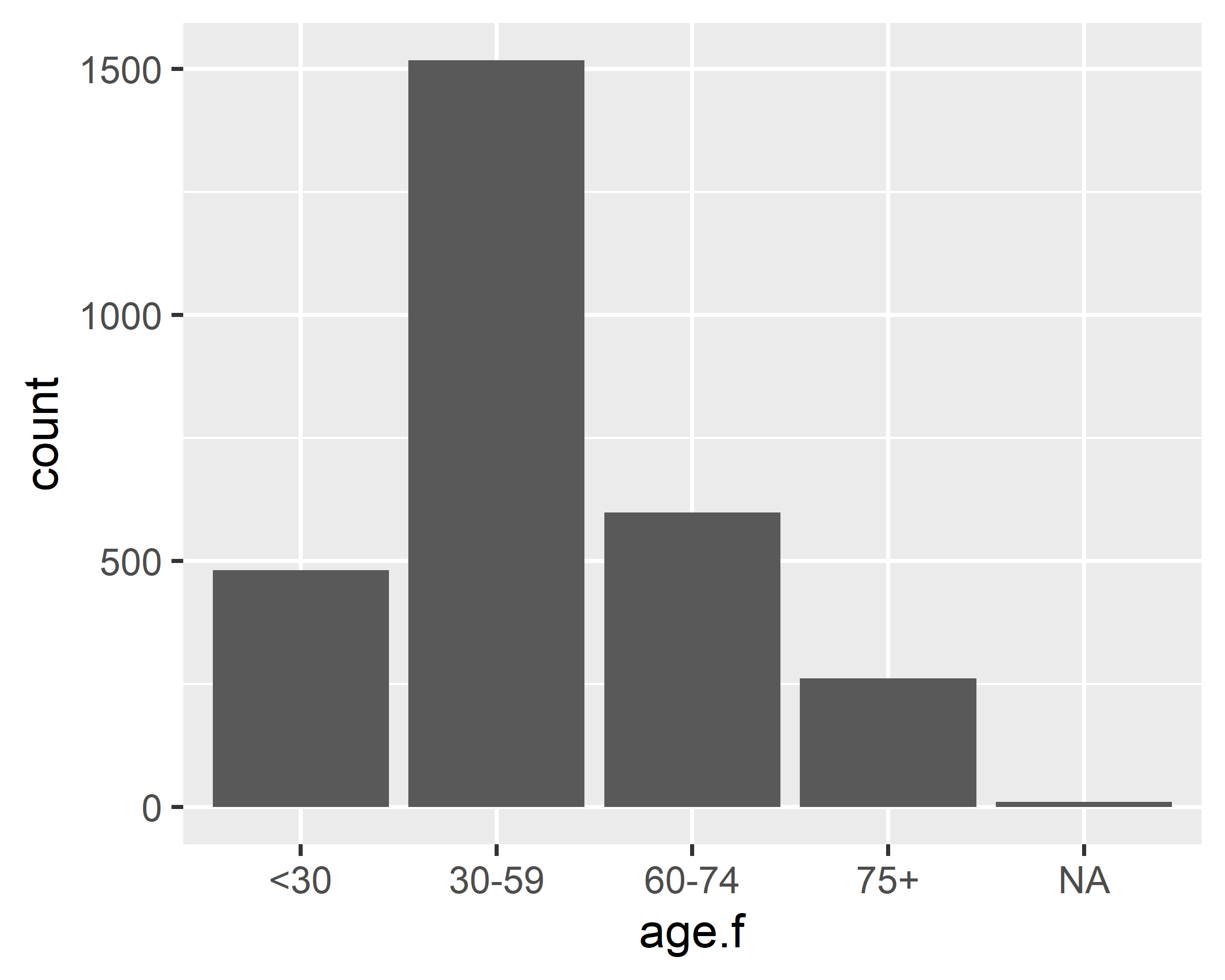
ggplot(data = gss.2016, mapping = aes(x=age.f)) + geom_bar() +
scale_x_discrete(na.translate = F)
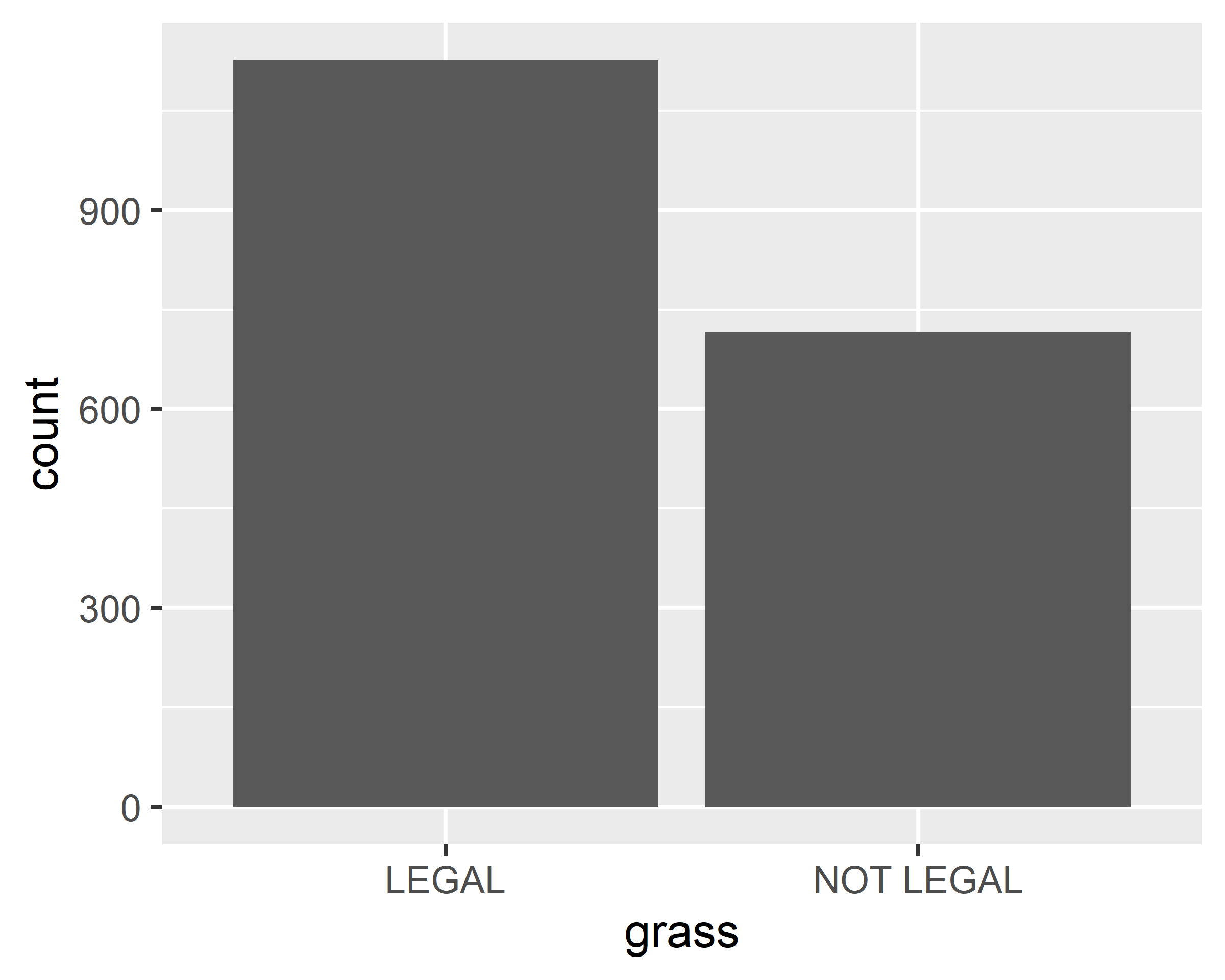
ggplot(data = gss.2016, mapping = aes(x=grass)) + geom_bar() +
scale_x_discrete(na.translate = F)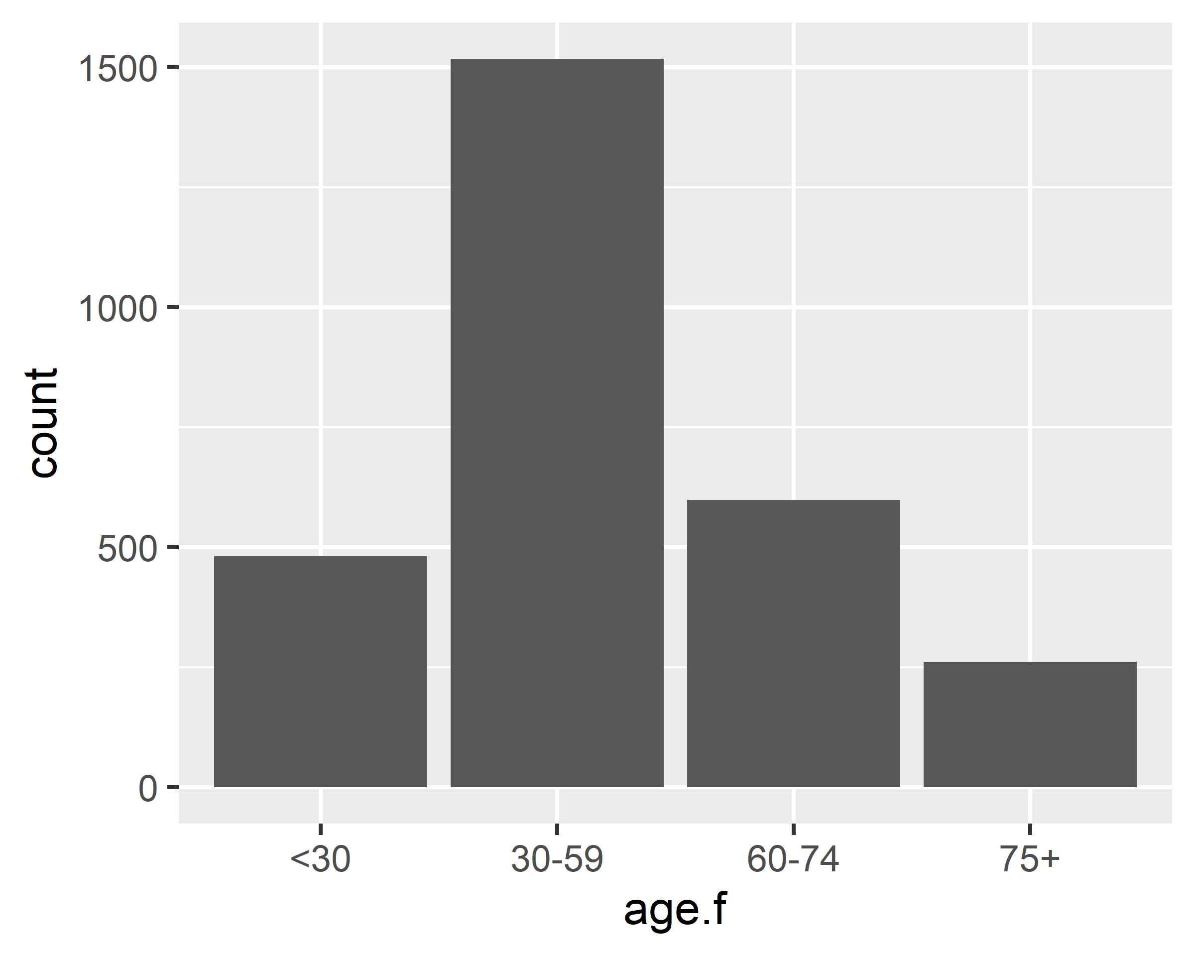
ggplot(data = gss.2016, mapping = aes(x=age.f, fill=age.f)) + geom_bar() +
  scale_x_discrete(na.translate = F)
ggplot(data = gss.2016, mapping = aes(x=grass, fill=grass)) + geom_bar() +
  scale_x_discrete(na.translate = F)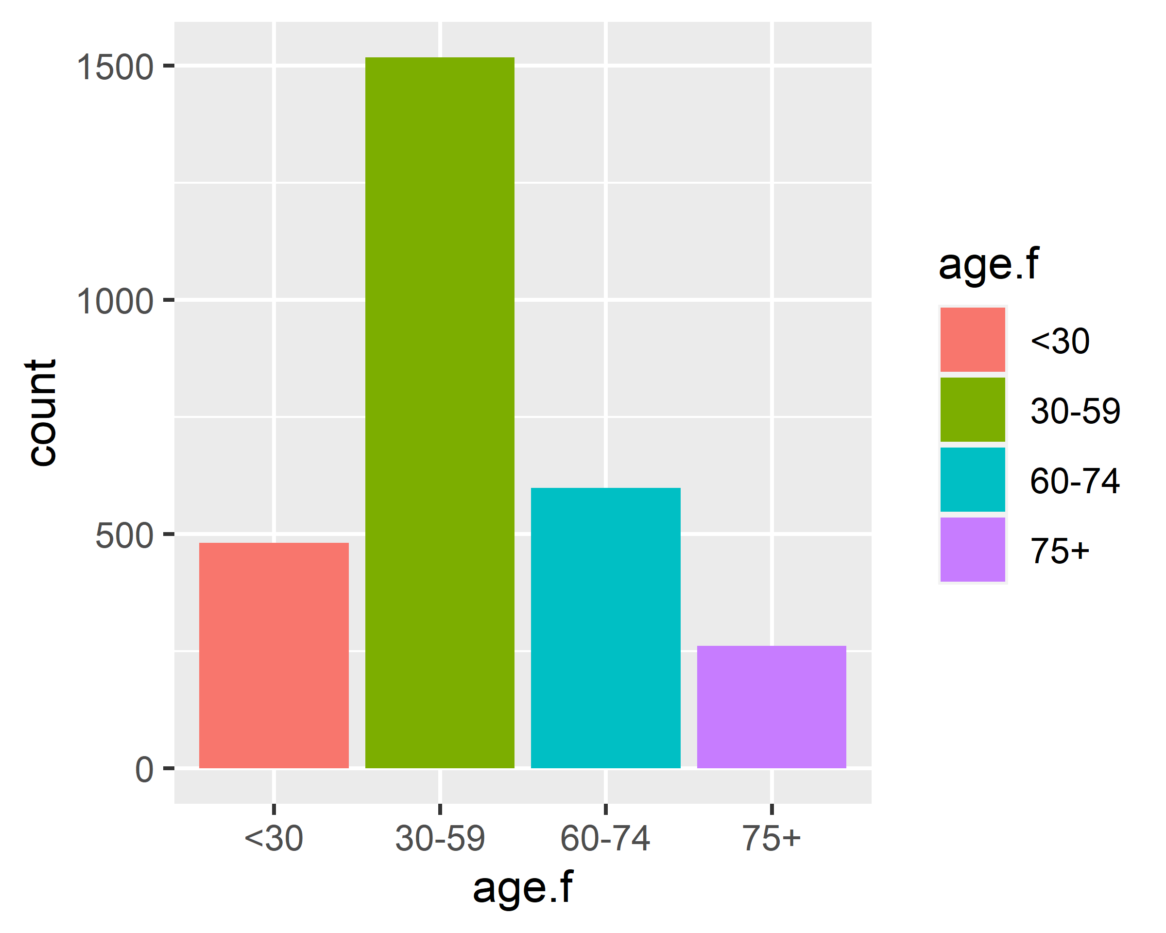
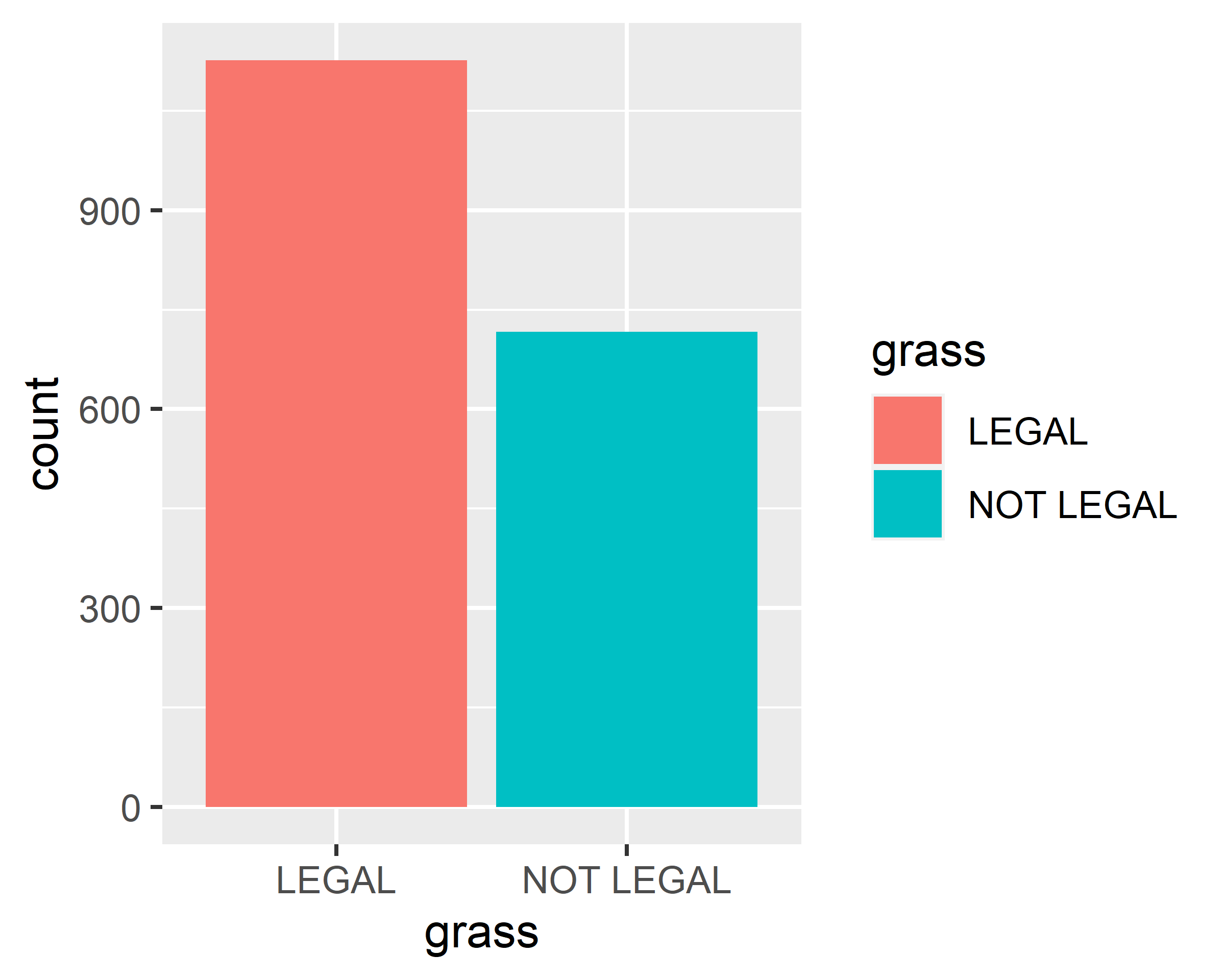
ggplot(data = gss.2016, mapping = aes(x=grass, fill=grass)) + geom_bar() +
scale_x_discrete(na.translate = F) +
scale_fill_manual(values = c("#78A678", "#7463AC"), guide=F)
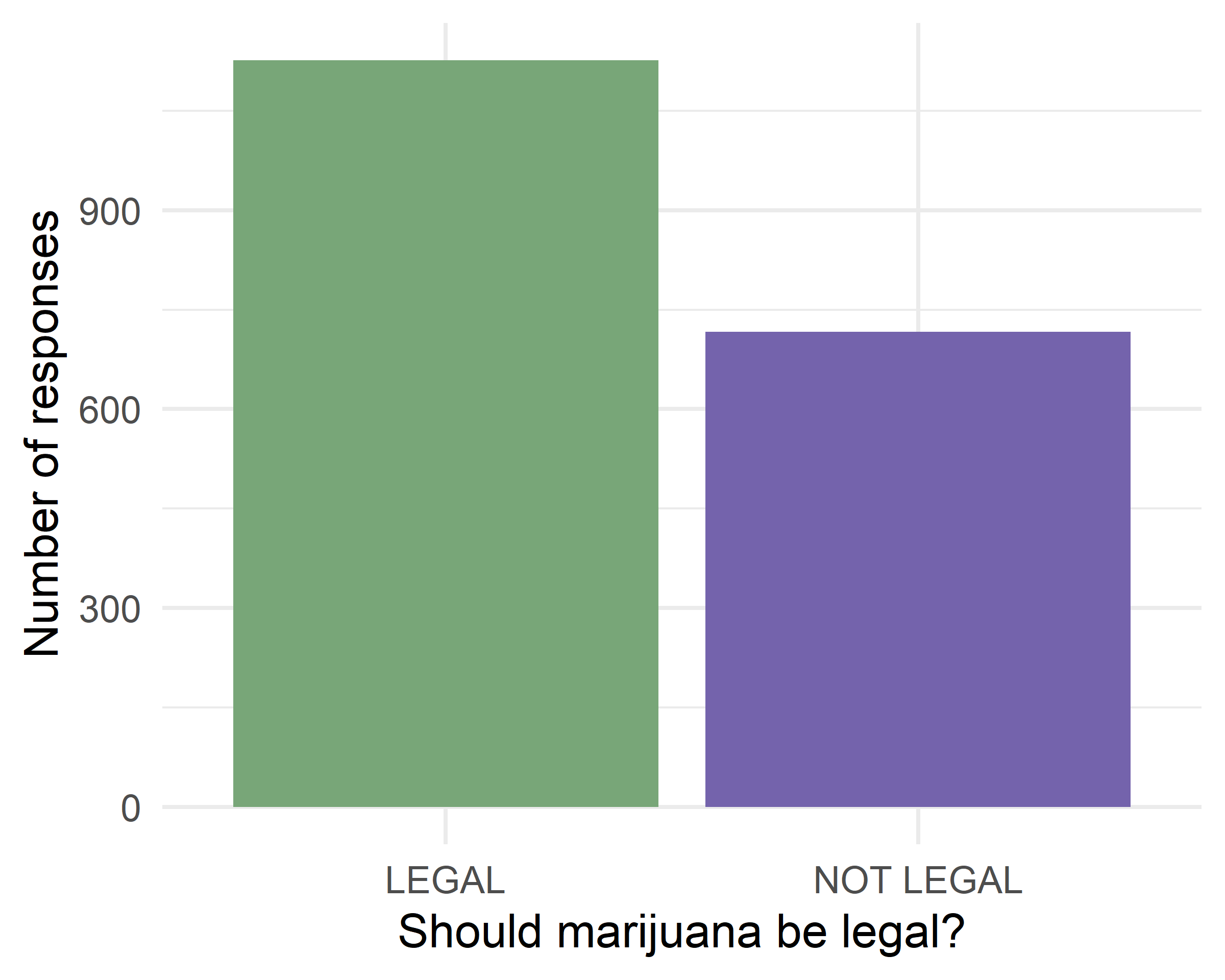
ggplot(data = gss.2016, mapping = aes(x=grass, fill=grass)) + geom_bar() +
scale_x_discrete(na.translate = F) +
scale_fill_manual(values = c("#78A678", "#7463AC"), guide=F) +
theme_minimal() +
labs(x="Should marijuana be legal?", y="Number of responses")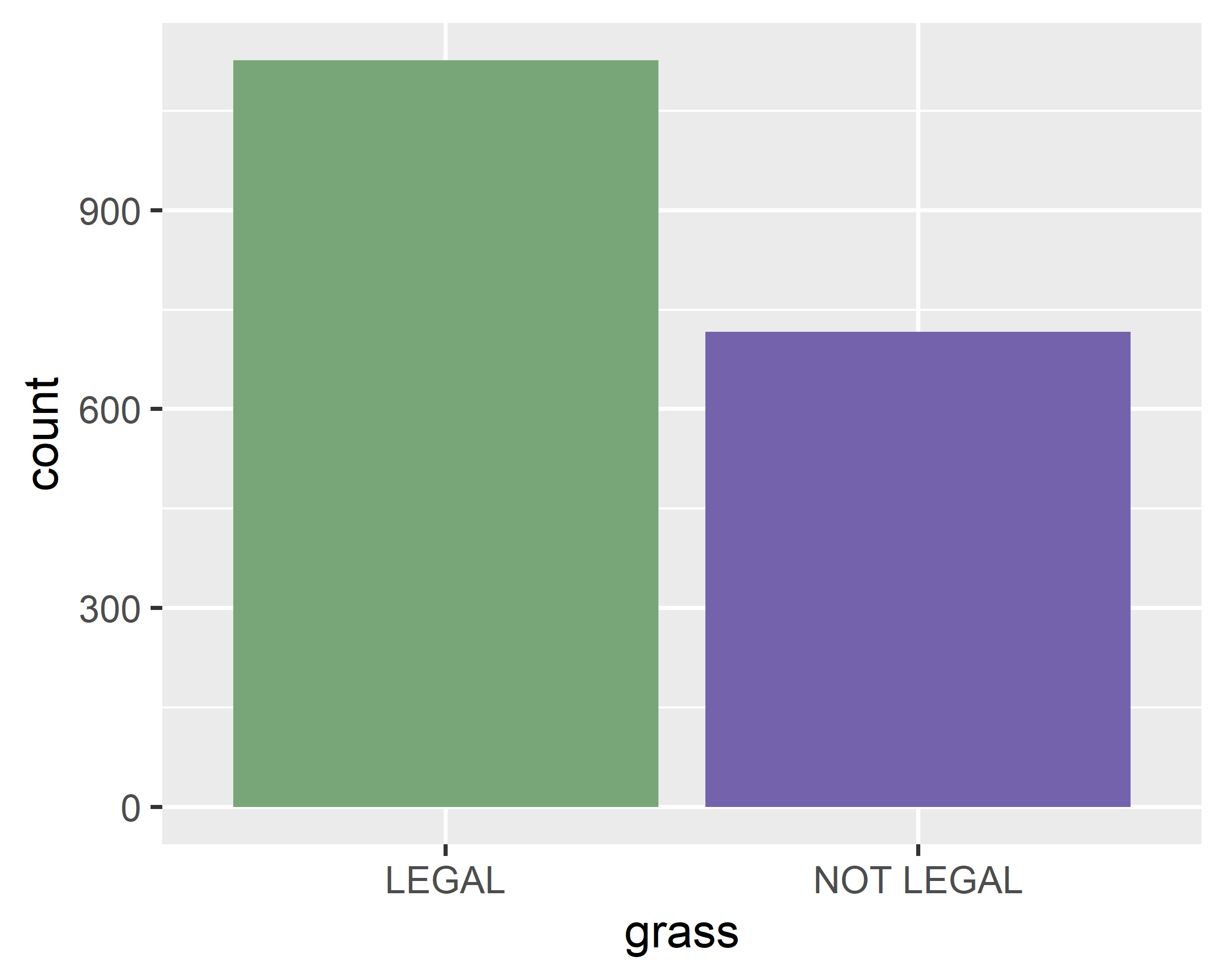
ggplot(data = gss.2016[!is.na(gss.2016$grass),],
       mapping = aes(x=age.f, fill=grass)) + geom_bar() +
  scale_x_discrete(na.translate = F)

ggplot(data = gss.2016[!is.na(gss.2016$grass),],
       mapping = aes(x=age.f, fill=grass)) + geom_bar(position = "fill") +
  scale_x_discrete(na.translate = F)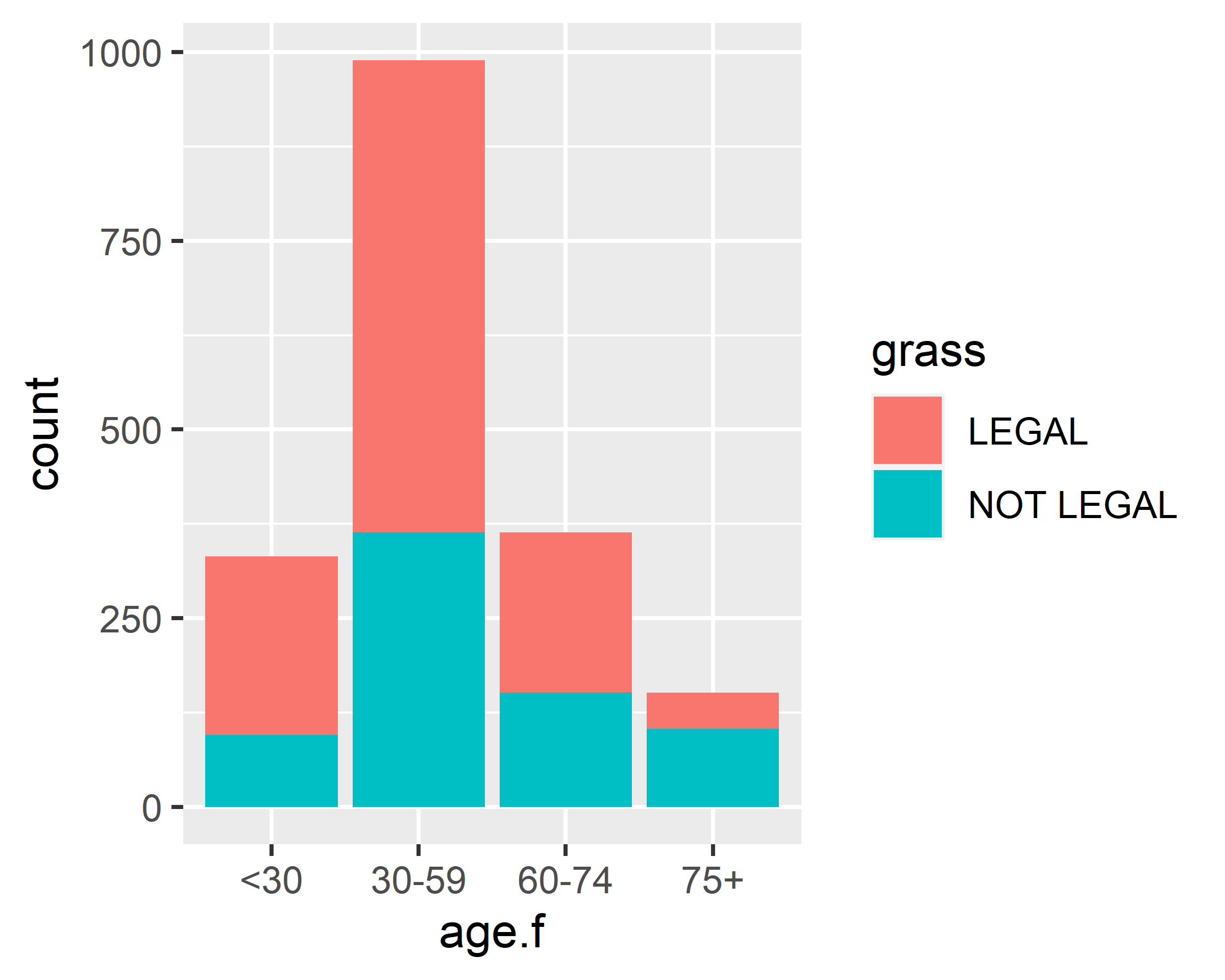
ggplot(data = gss.2016[!is.na(gss.2016$grass),],
       mapping = aes(x=age.f, fill=grass)) + geom_bar(position = "dodge") +
  scale_x_discrete(na.translate = F) +
    labs(x="Should marijuana be legal?", y="Number of responses", fill="Legal")
ggplot(data = gss.2016[!is.na(gss.2016$age.f),],
       mapping = aes(x=grass, fill=age.f)) + geom_bar(position = "dodge") +
  scale_x_discrete(na.translate = F) +
    labs(x="Should marijuana be legal?", y="Number of responses", fill="Age")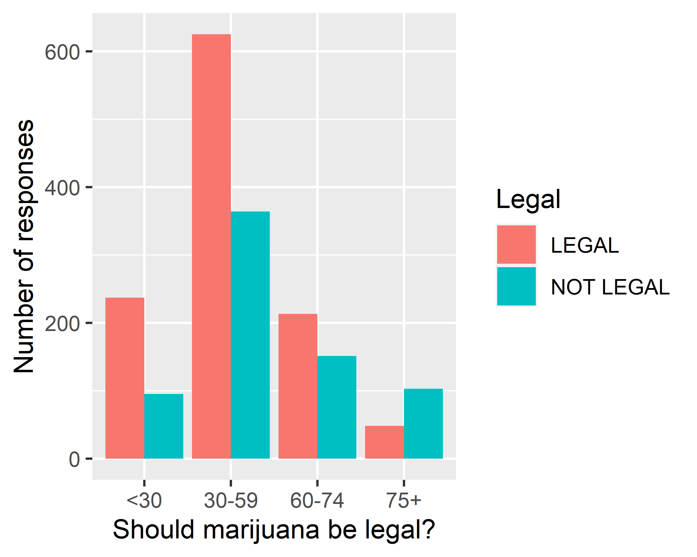
3.5.2.2 Histogram
Please study carefully the following codes and outputs:
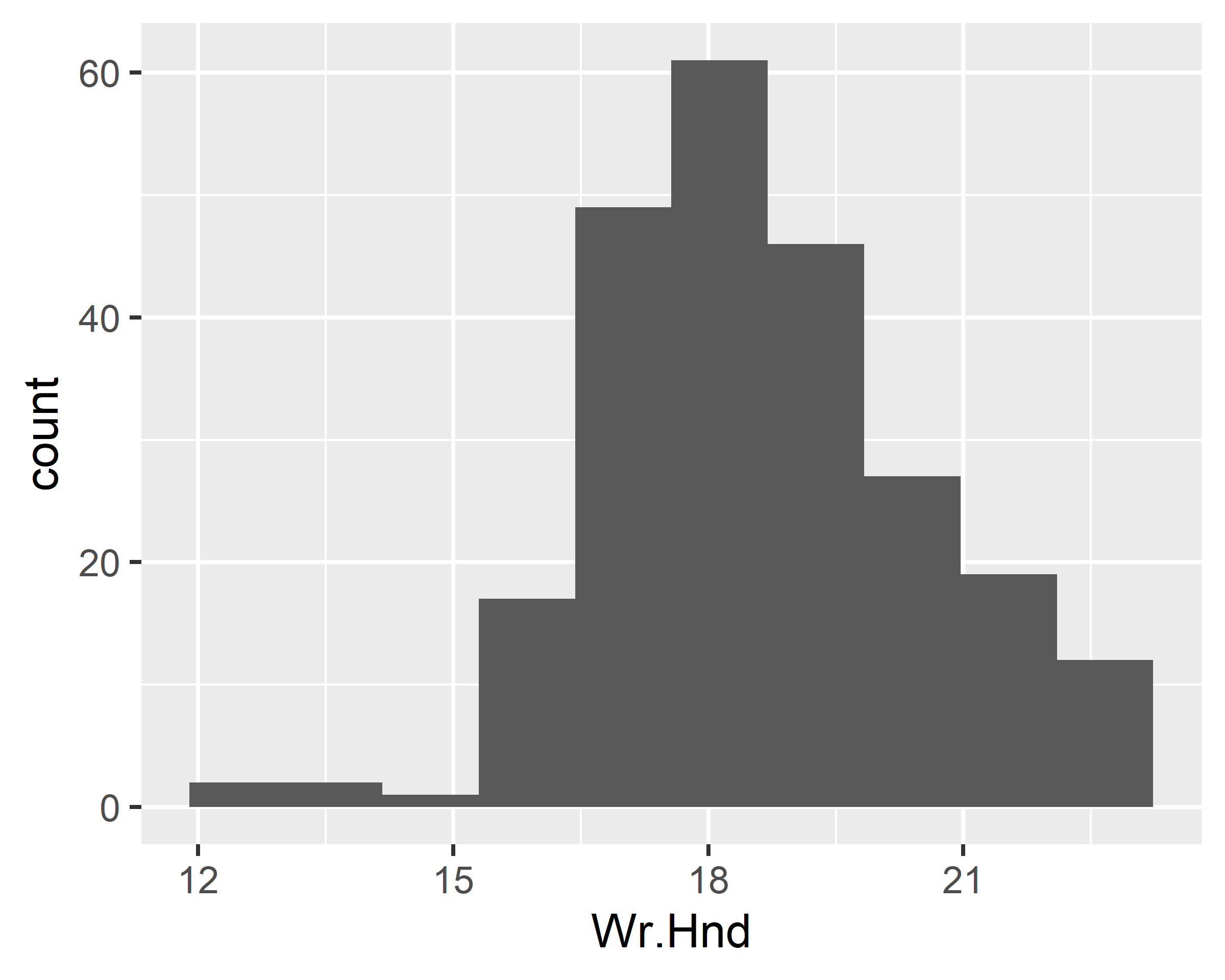
ggplot(data = survey, mapping = aes(x=Wr.Hnd)) + geom_histogram()
ggplot(data = survey, mapping = aes(x=Wr.Hnd)) + geom_histogram(bins = 10)
ggplot(data = survey, mapping = aes(x=Wr.Hnd)) +
geom_histogram(bins = 10, fill="lightblue", colour="blue")
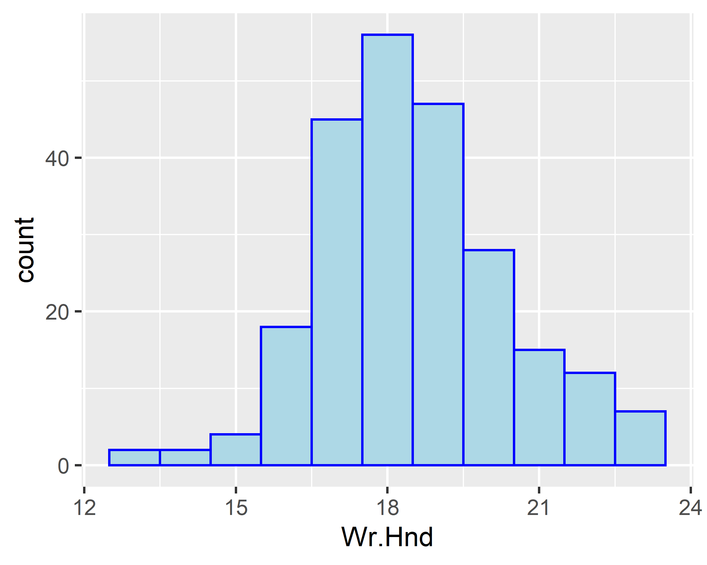
ggplot(data = survey, mapping = aes(x=Wr.Hnd)) +
geom_histogram(binwidth = 1, fill="lightblue", colour="blue")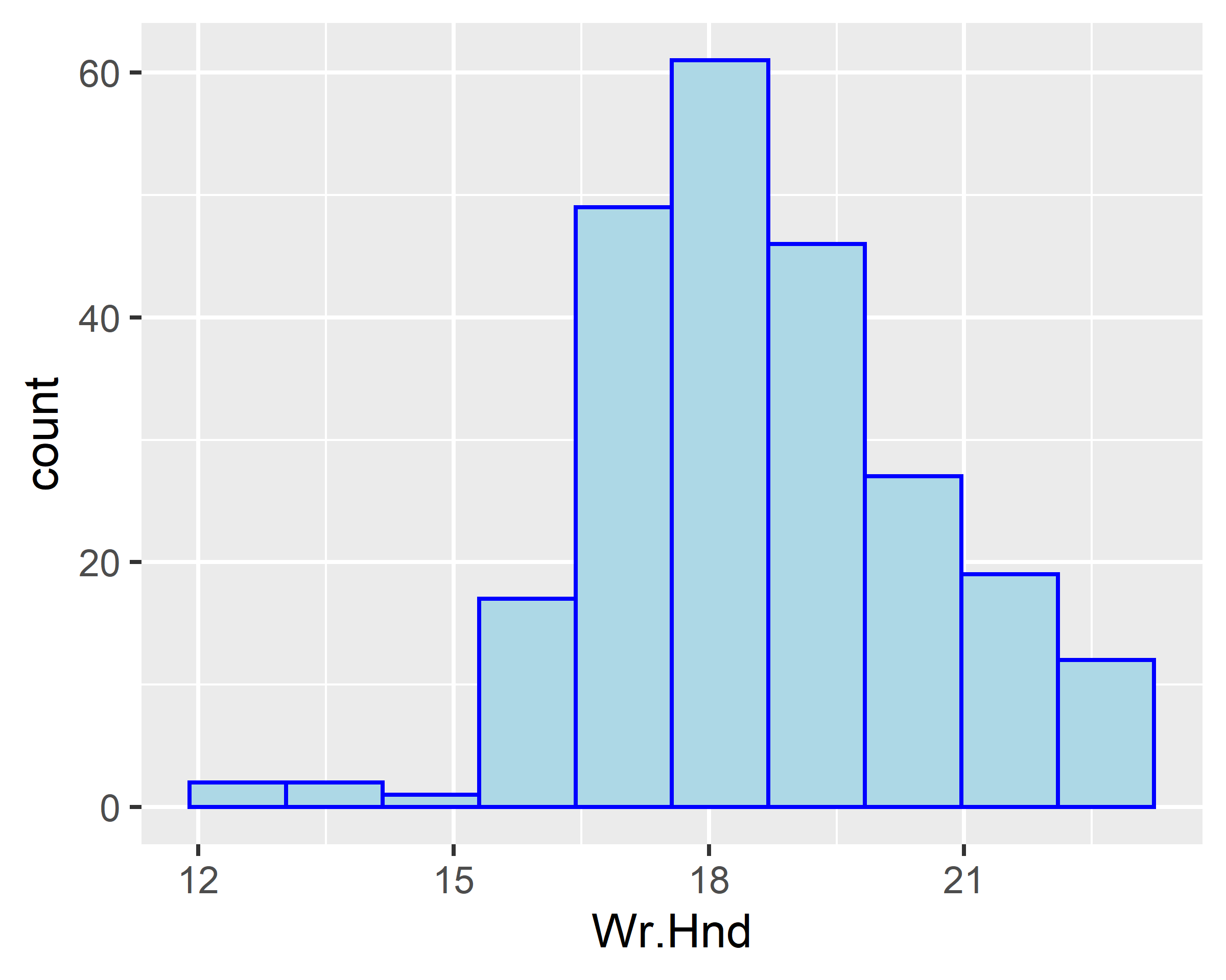
ggplot(data = survey, mapping = aes(x=Wr.Hnd)) +
geom_histogram(binwidth = 1, fill="lightblue", colour="blue") +
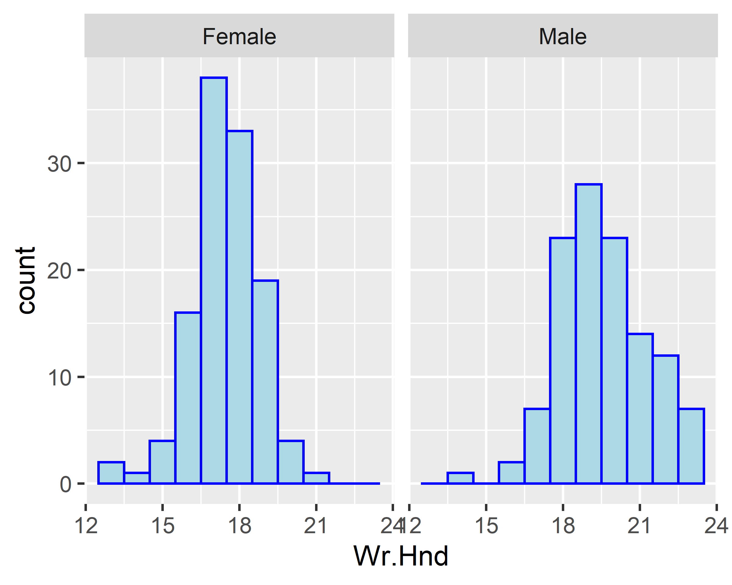
facet_wrap(~Sex)
ggplot(data = survey[!is.na(survey$Sex),], mapping = aes(x=Wr.Hnd)) +
geom_histogram(binwidth = 1, fill="lightblue", colour="blue") +
facet_wrap(~Sex)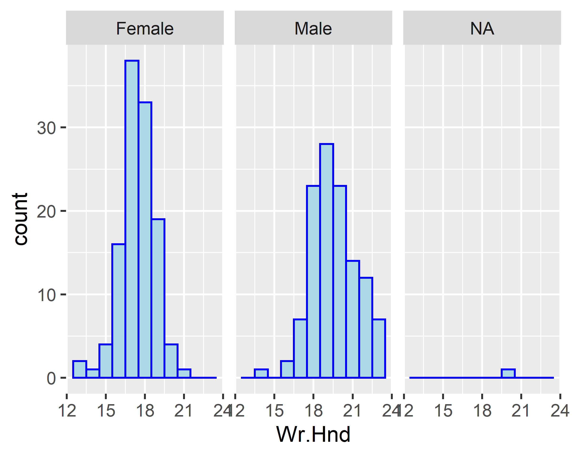
ggplot(data = survey[!is.na(survey$Sex),], mapping = aes(x=Wr.Hnd)) +
  geom_histogram(binwidth = 1, fill="lightblue", colour="blue") +
  facet_wrap(~Sex, ncol=1)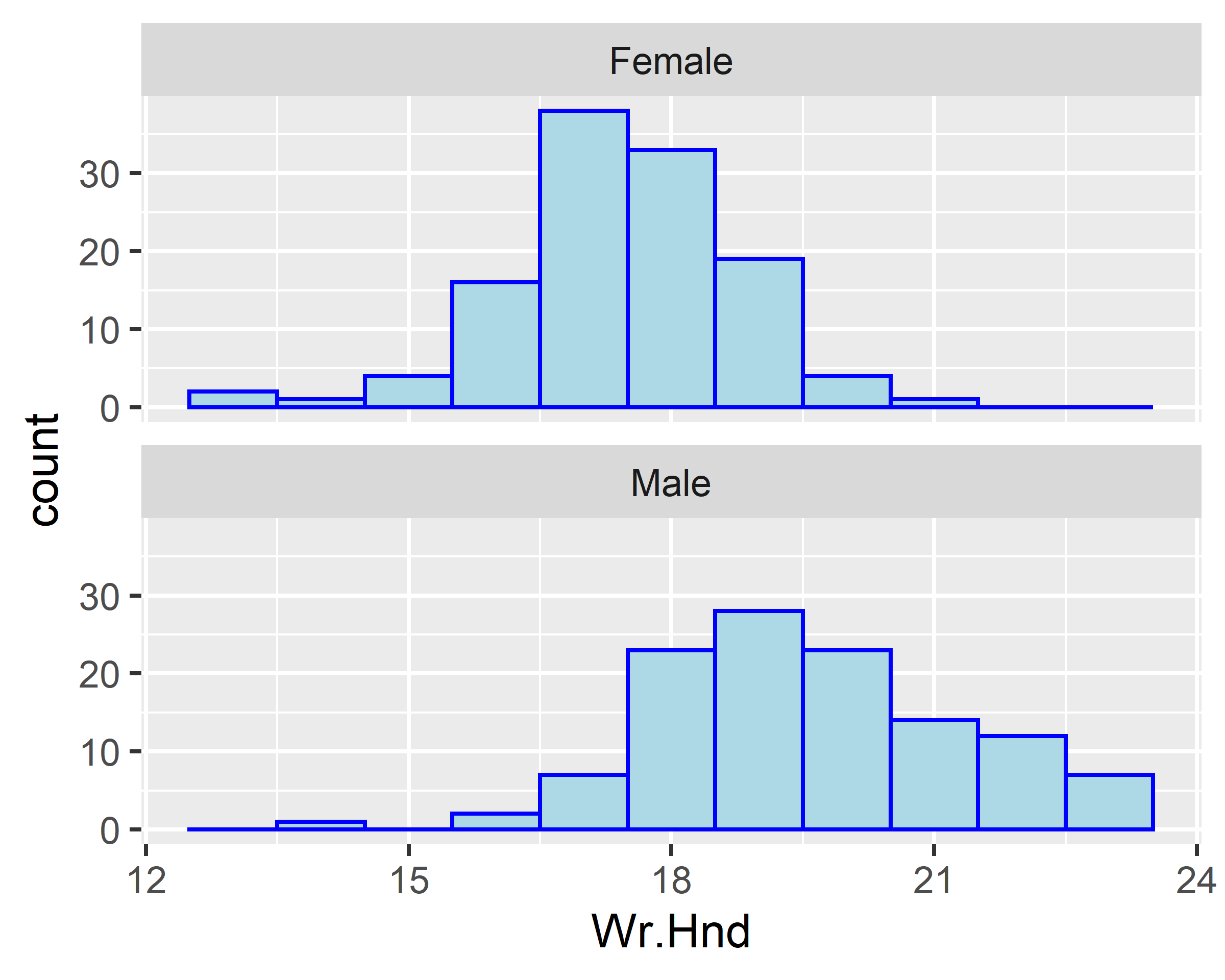
3.5.2.3 Scatterplot
ggplot(data = survey, mapping = aes(x=Wr.Hnd, y=Height)) +
  geom_point()
ggplot(data = survey, mapping = aes(x=Wr.Hnd, y=Height, color=Sex)) +
  geom_point()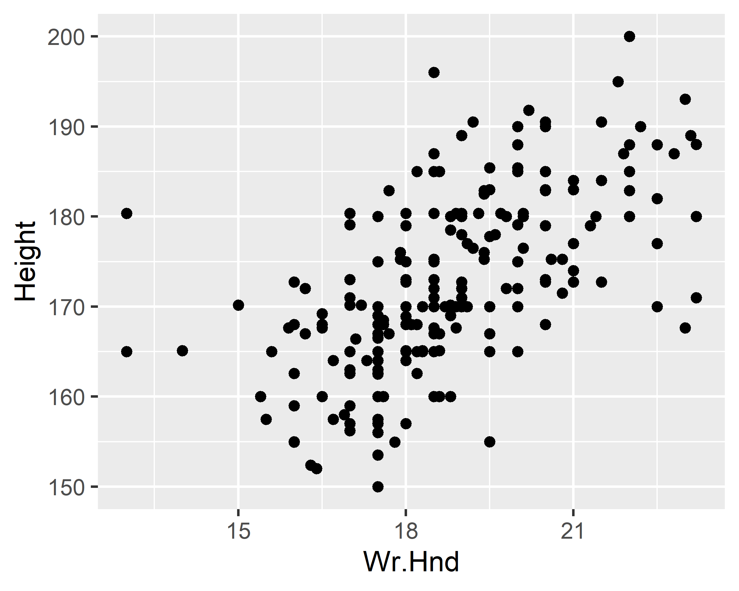
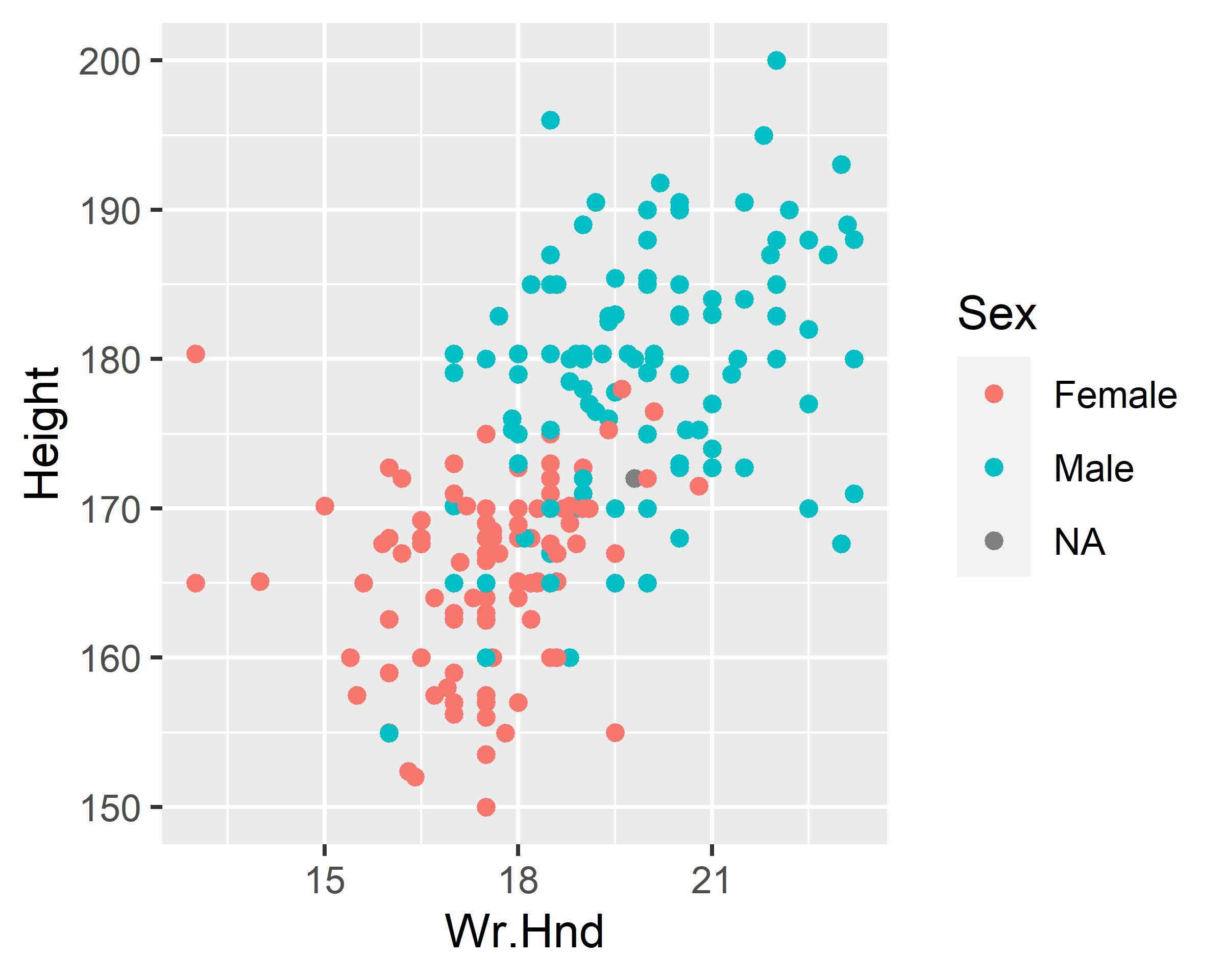
ggplot(data = survey, mapping = aes(x=Wr.Hnd, y=Height, color=Sex)) +
geom_point() + scale_color_discrete(na.translate=F)
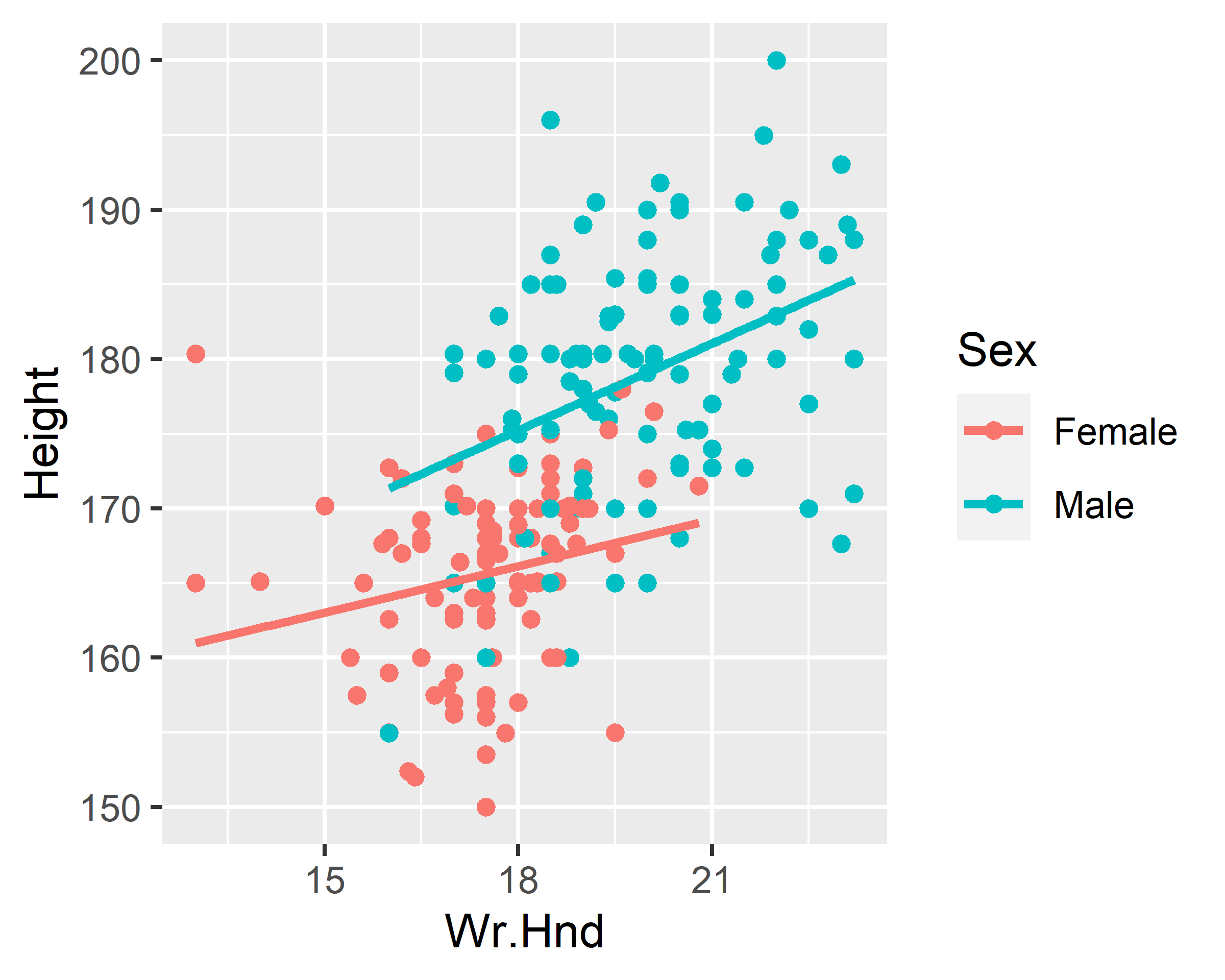
ggplot(data = survey, mapping = aes(x=Wr.Hnd, y=Height, color=Sex)) +
geom_point() + scale_color_discrete(na.translate=F) +
geom_smooth(se = F, method = lm)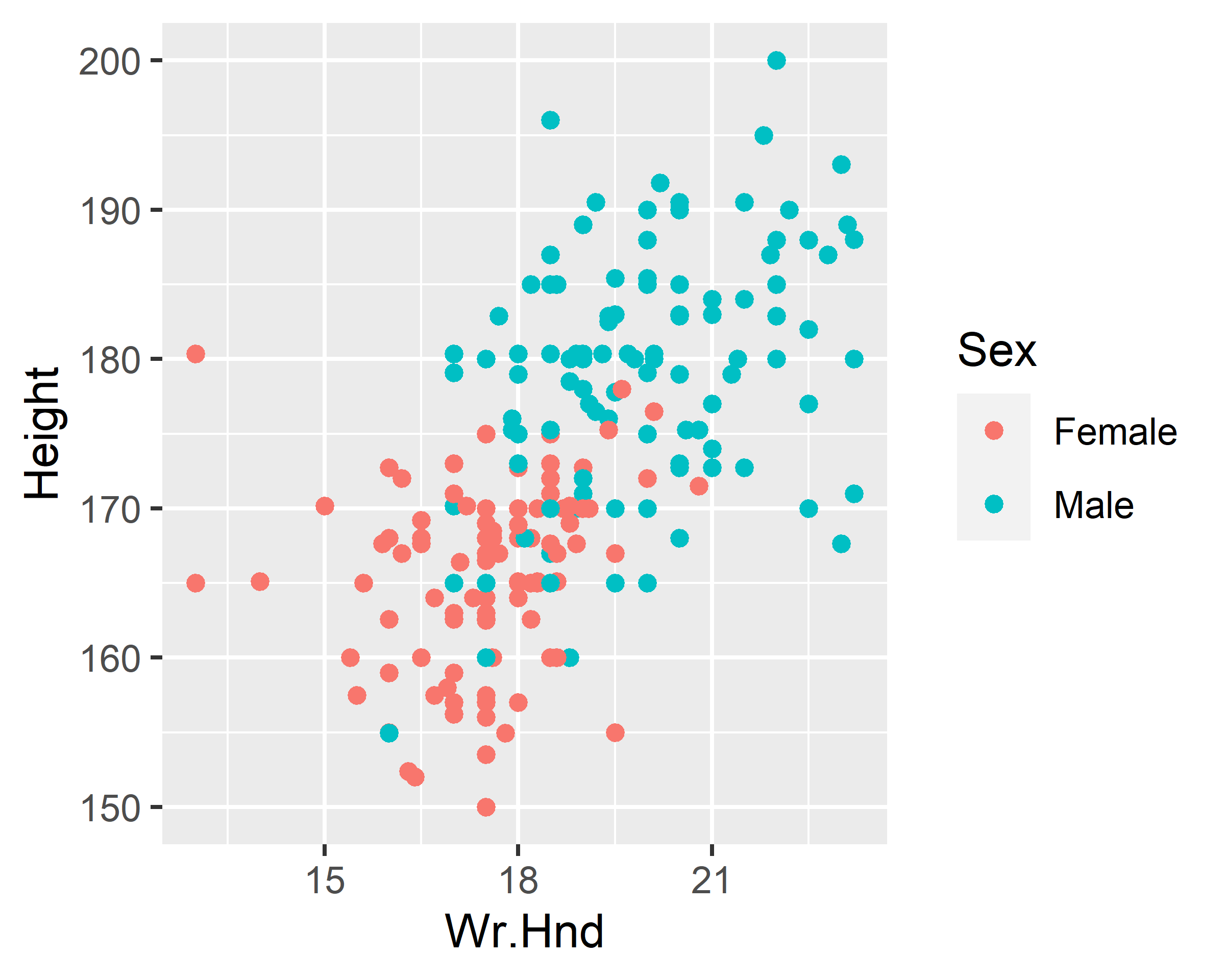
3.5.2.4 Box plot
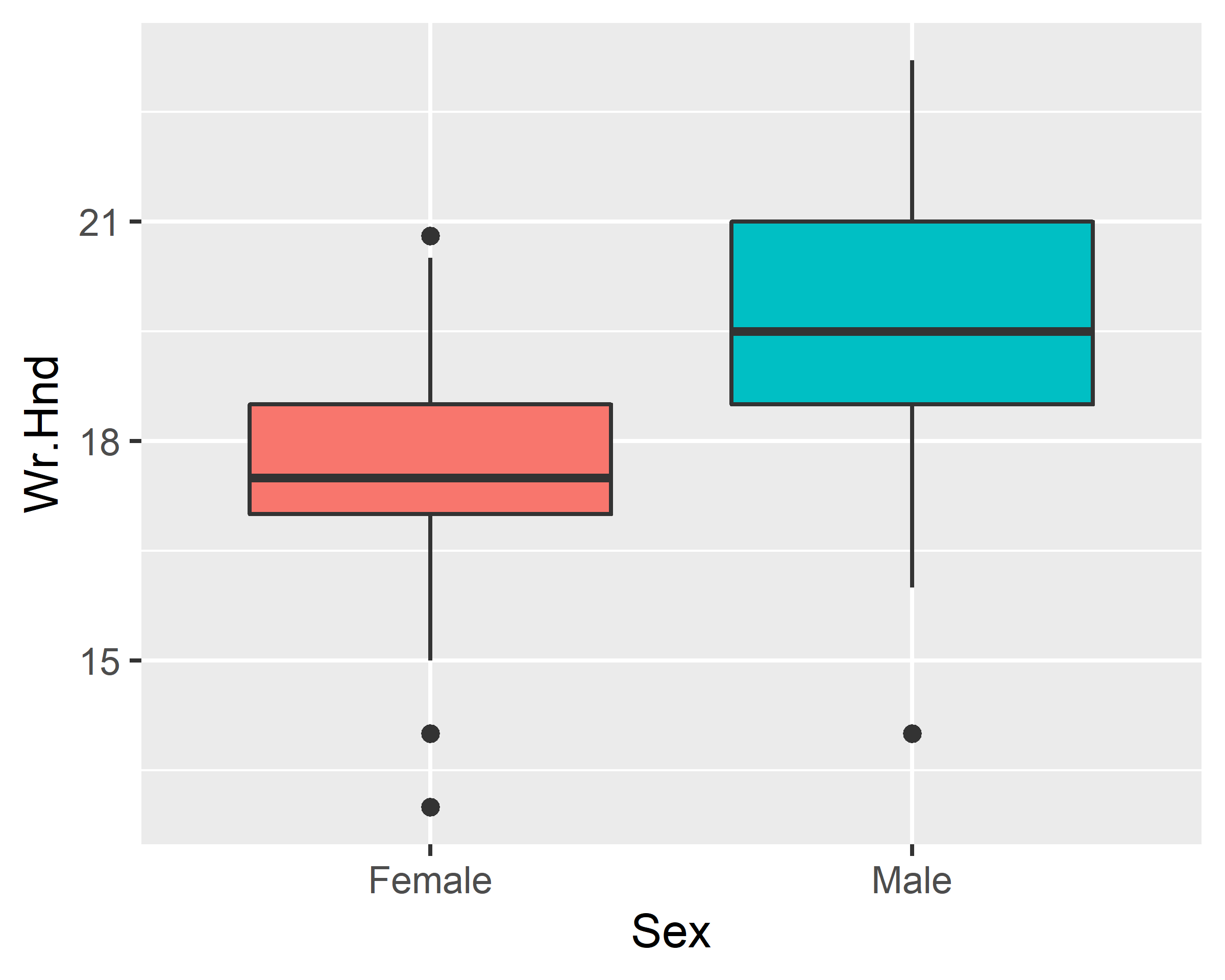
ggplot(data = survey, mapping = aes(x=Sex, y=Wr.Hnd)) +
  geom_boxplot()
ggplot(data = survey, mapping = aes(x=Sex, y=Wr.Hnd)) +
  geom_boxplot() + scale_x_discrete(na.translate=F)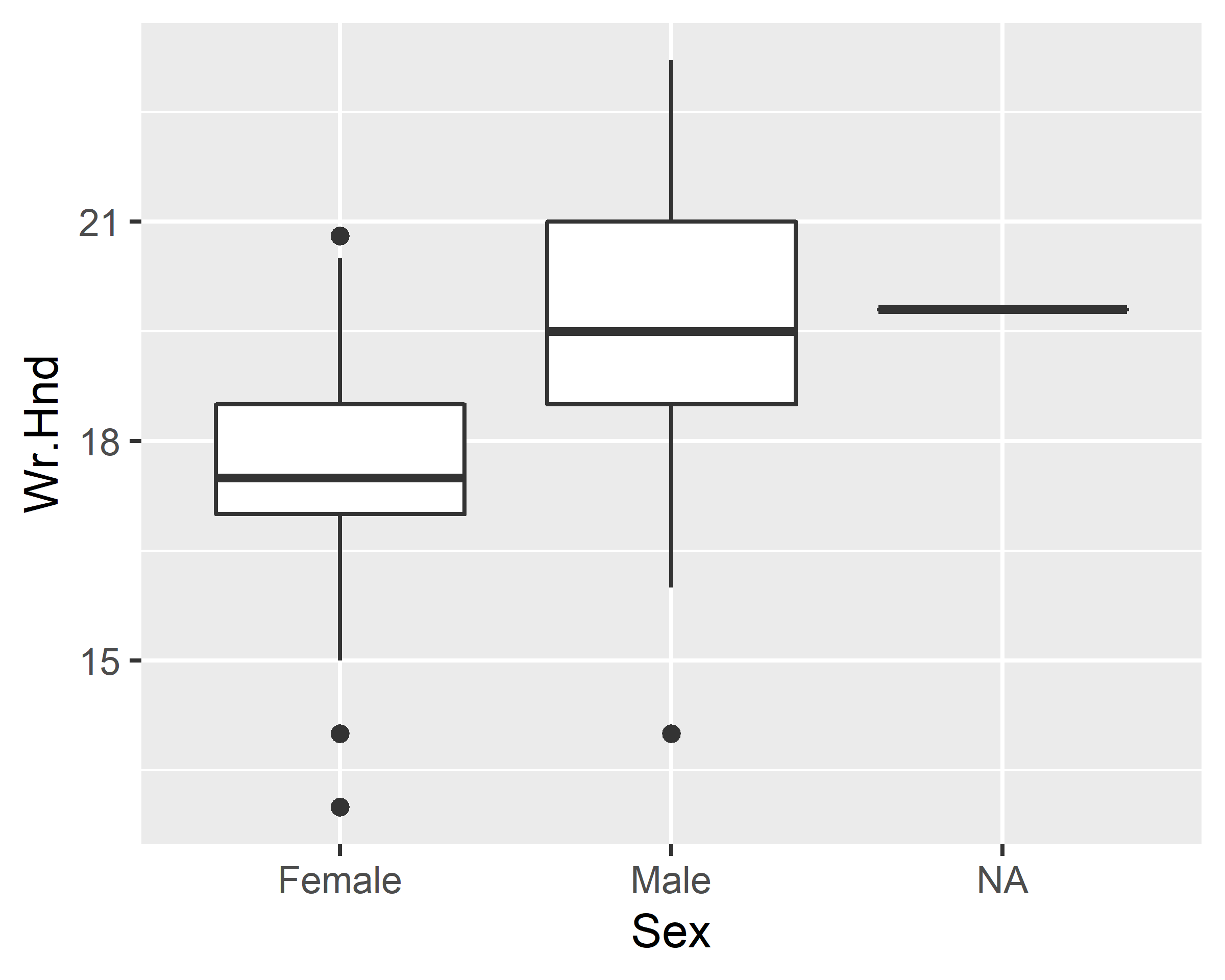
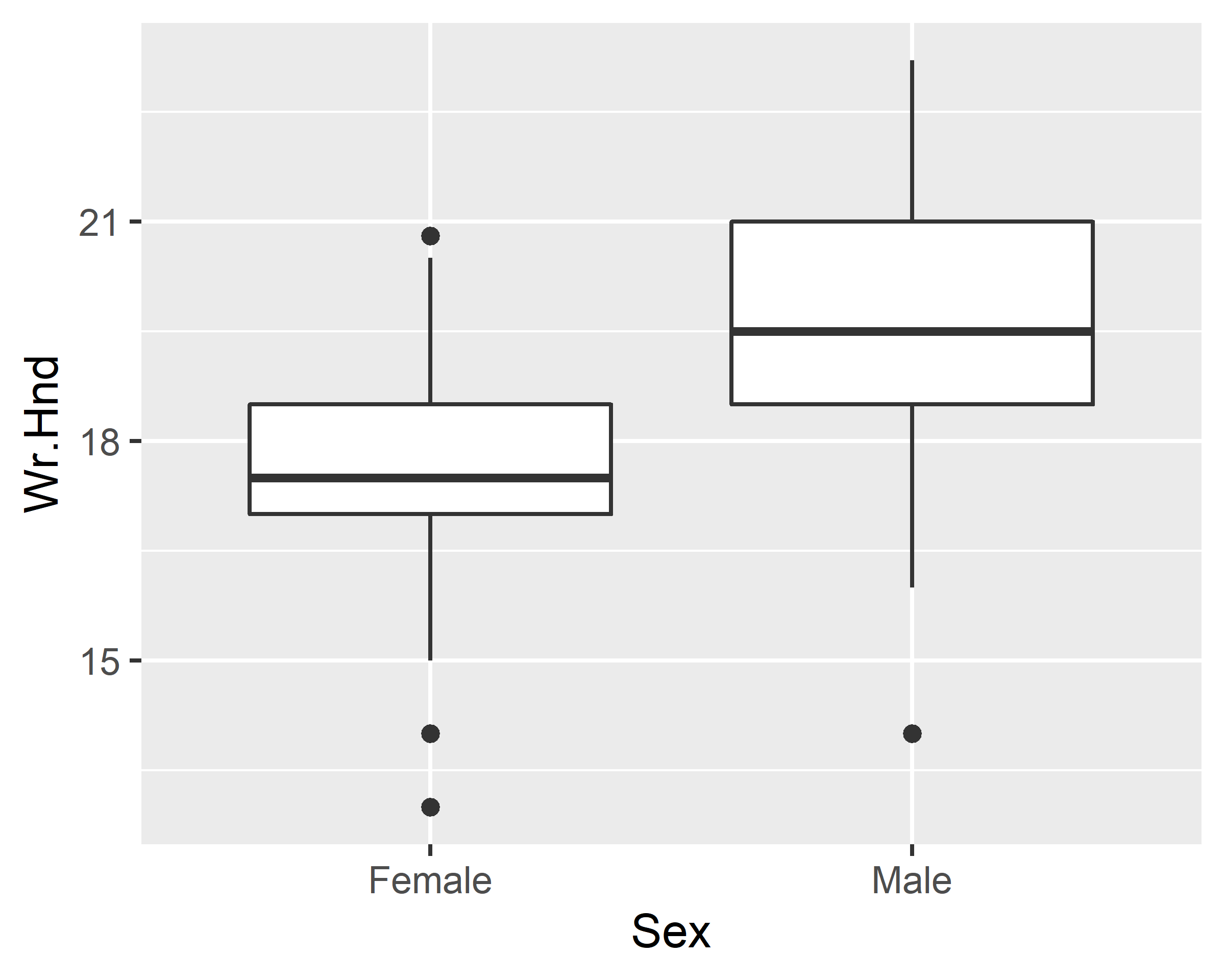
ggplot(data = survey, mapping = aes(x=Sex, y=Wr.Hnd, fill=Sex)) +
  geom_boxplot() + scale_x_discrete(na.translate=F)

ggplot(data = survey, mapping = aes(x=Sex, y=Wr.Hnd, fill=Sex)) +
  geom_boxplot() + scale_x_discrete(na.translate=F) +
scale_fill_discrete(guide=F) 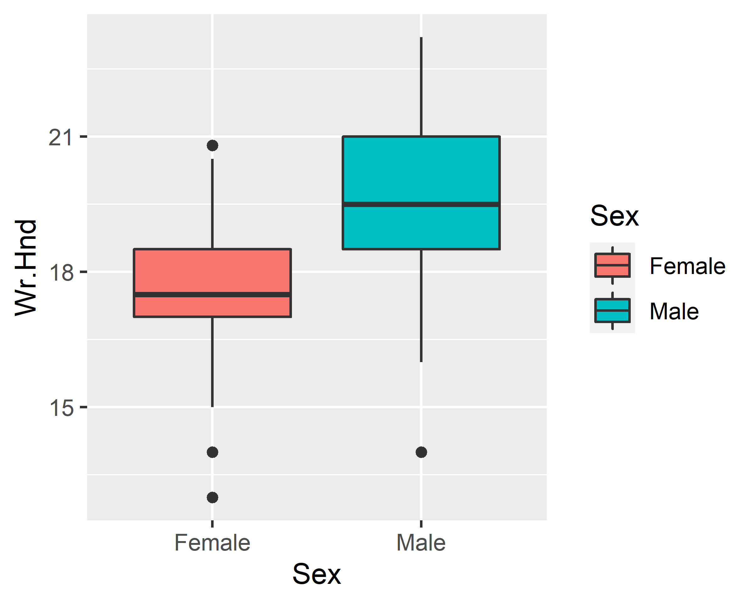
3.5.2.5 Stripchart
ggplot(data = survey, mapping = aes(x=1, y=Wr.Hnd)) +
  geom_jitter() + scale_x_discrete(na.translate=F)
ggplot(data = survey, mapping = aes(x=Sex, y=Wr.Hnd)) +
  geom_jitter() + scale_x_discrete(na.translate=F)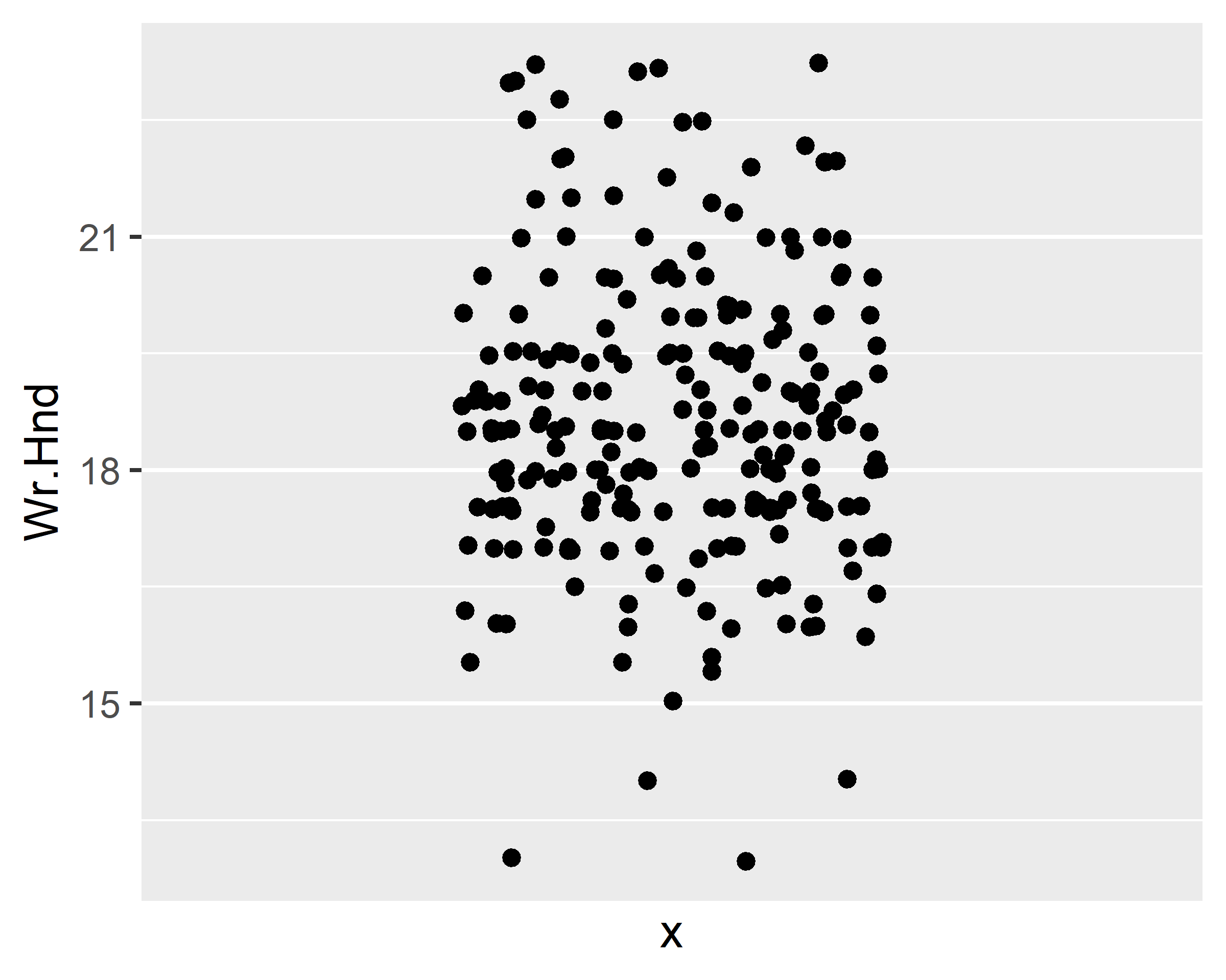
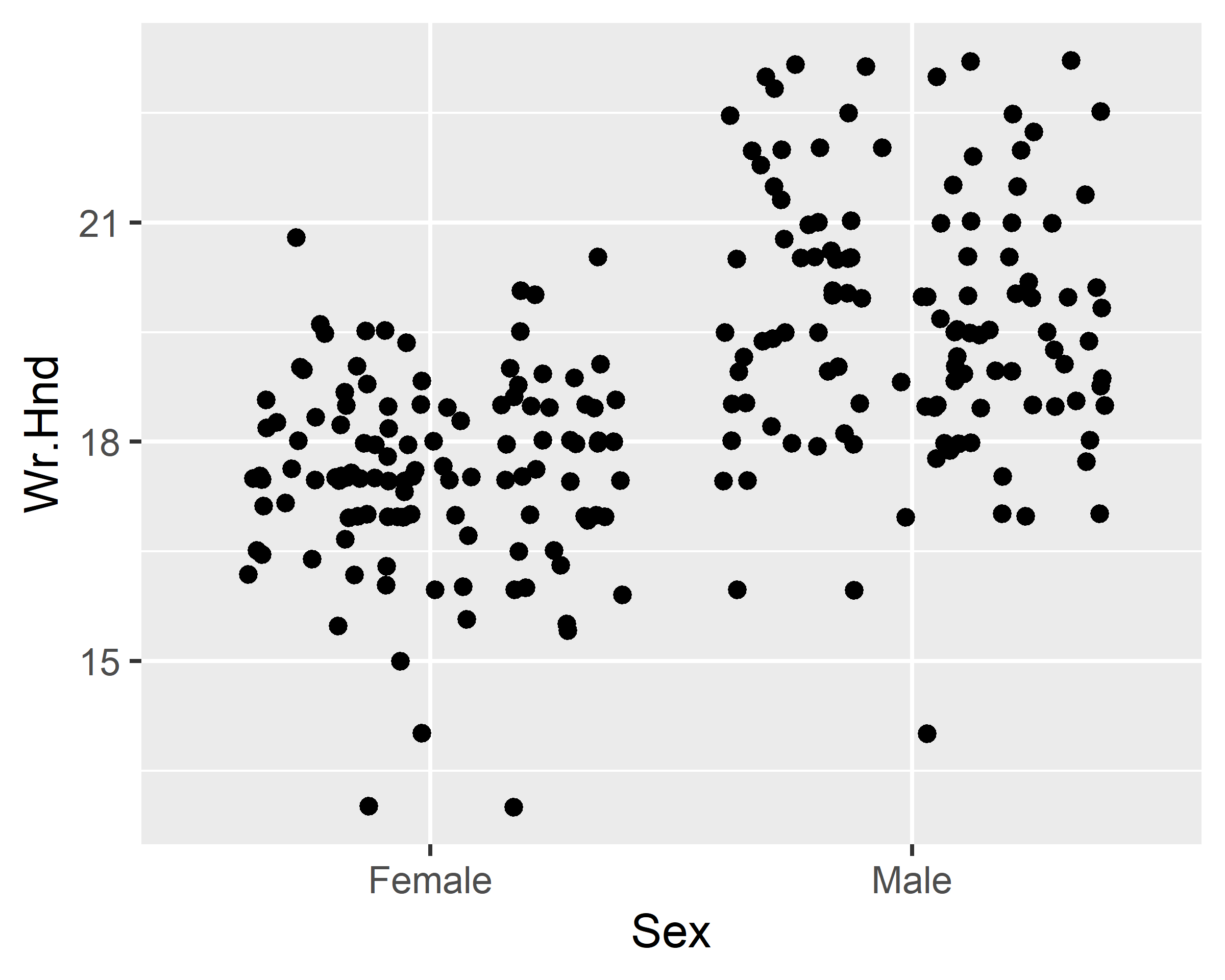
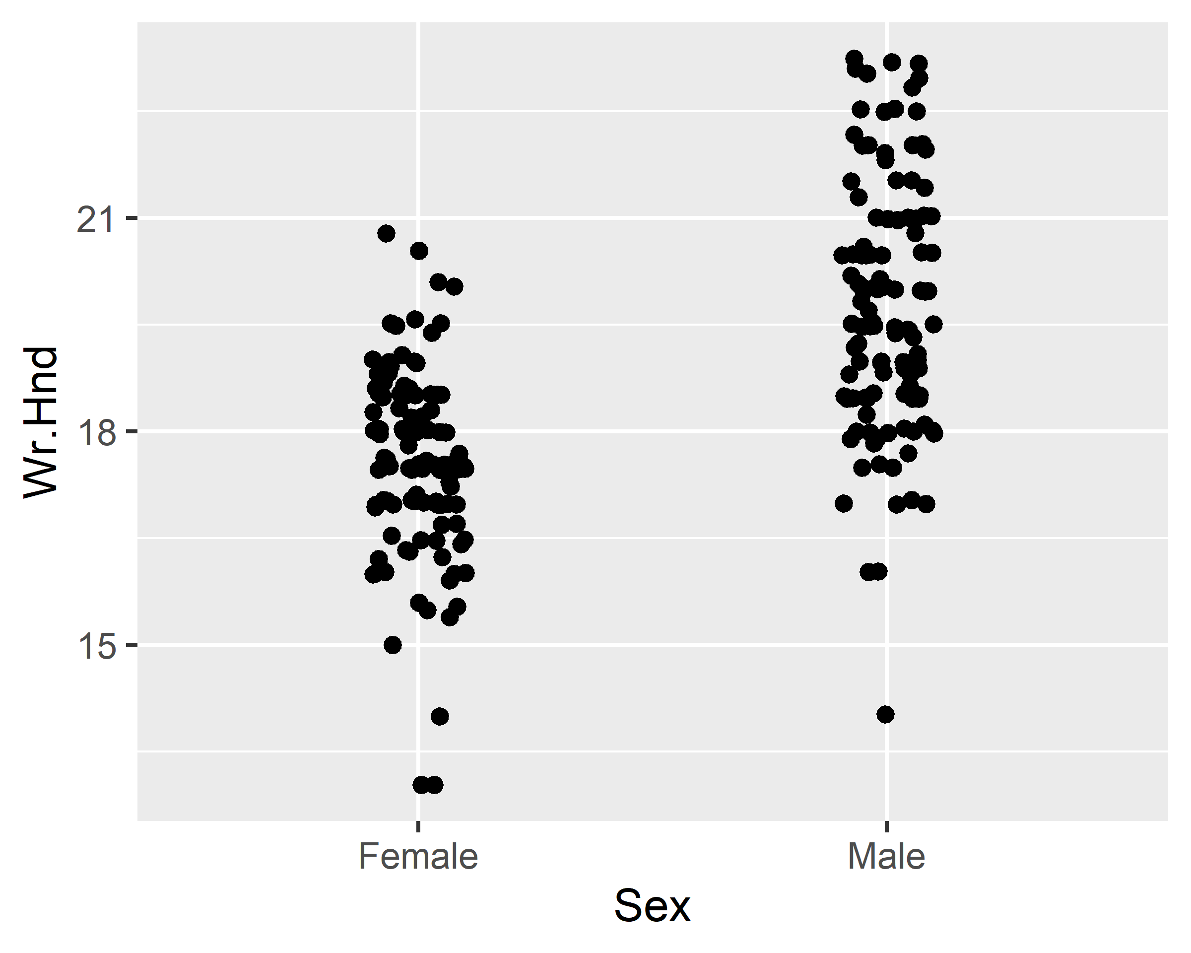
ggplot(data = survey, mapping = aes(x=Sex, y=Wr.Hnd)) +
geom_jitter(width = 0.1) + scale_x_discrete(na.translate=F)
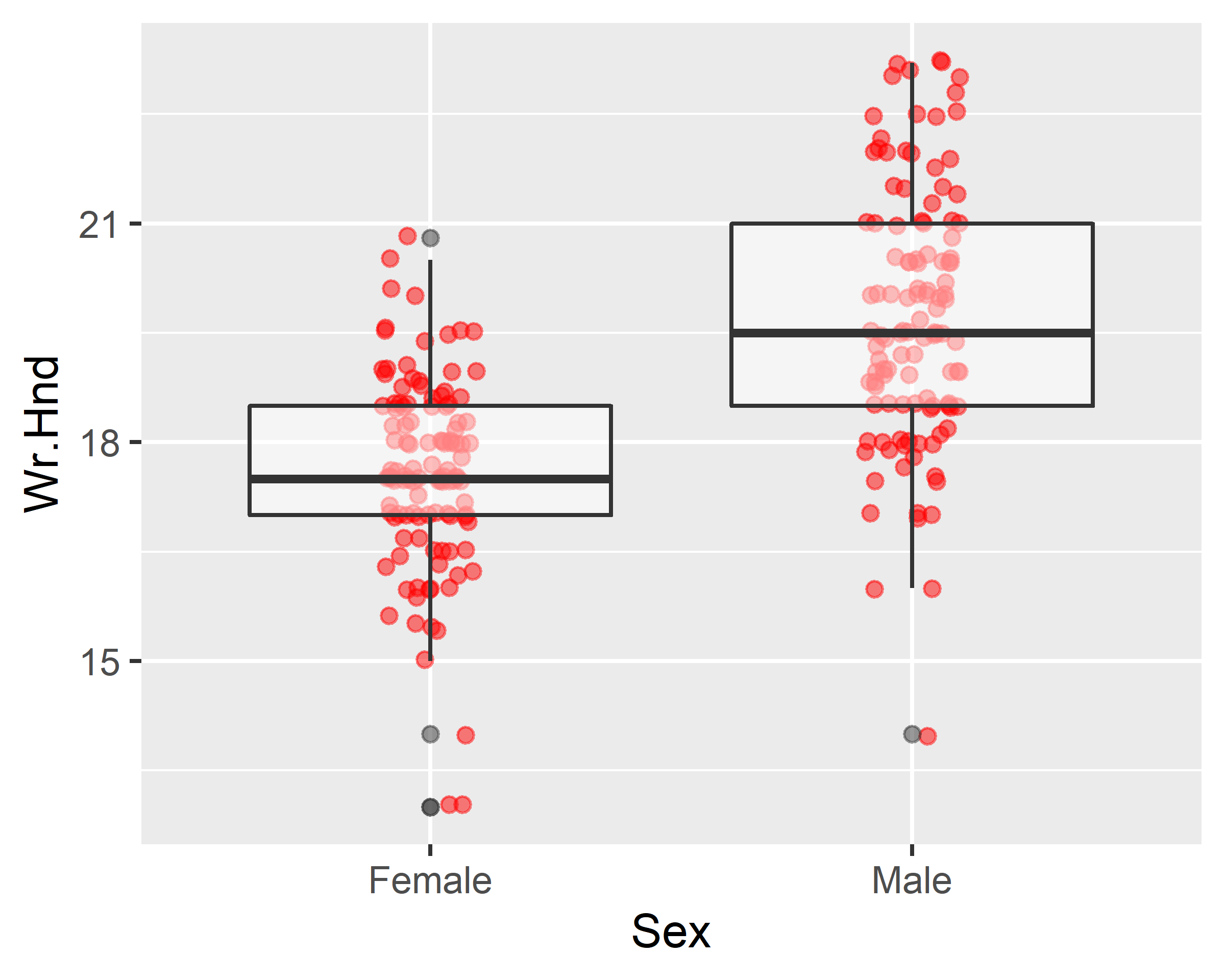
ggplot(data = survey, mapping = aes(x=Sex, y=Wr.Hnd)) +
geom_jitter(width = 0.1, alpha=0.5, color="red") +
scale_x_discrete(na.translate=F) +
geom_boxplot(alpha=0.5)